

| LTTng-UST Analyses | ||
|---|---|---|
|
|
|
|
| LTTng Kernel Analysis | Trace synchronization | |
The Userspace traces are taken on an application level. With kernel traces, you know what events you will have as the domain is known and cloistered. Userspace traces can contain pretty much anything. Some analyses are offered if certain events are enabled.
The Flame Chart view allows the user to visualize the call stack per thread over time, if the application and trace provide this information.
To open this view go in Window -> Show View, if in the eclipse plug-in then click Other... and select Tracing/Flame Chart in the list. The view shows the call stack information for the currently selected trace. Conversely, you can select a trace and expand it in the Project Explorer then expand LTTng-UST CallStack Analysis (the trace must be loaded) and open Flame Chart.
The table on the left-hand side of the view shows the threads and call stack. The function name, depth, entry and exit time and duration are shown for the call stack at the selected time.
Double-clicking on a function entry in the table will zoom the time graph to the selected function's range of execution.
The time graph on the right-hand side of the view shows the call stack state graphically over time. The function name is visible on each call stack event if size permits. The color of each call stack event is randomly assigned based on the function name, allowing for easy identification of repeated calls to the same function.
Clicking on the time graph will set the current time and consequently update the table with the current call stack information.
Shift-clicking on the time graph will select a time range. When the selection is a time range, the begin time is used to update the stack information.
Double-clicking on a call stack event will zoom the time graph to the selected function's range of execution.
Clicking the Select Next State Change or Select Previous State Change or using the left and right arrows will navigate to the next or previous call stack event, and select the function currently at the top of the call stack. Note that pressing the Shift key at the same time will update the selection end time of the current selection.
Clicking the
Configure how addresses are mapped to function names (
 ) icon will open the symbol providers dialog. Depending on the available symbol providers for the given trace, you can specify: 1) a text or binary file containing mappings from function addresses to function names or 2) the root location of the binaries of the trace target. If the call stack provider for the current trace type only provides function addresses, a mapping file will be required to get the function names in the view. See the following sections for an example with LTTng-UST traces.
There is support in the LTTng-UST integration plugin to display the callstack of applications traced with the liblttng-ust-cyg-profile.so library (see the liblttng-ust-cyg-profile man page for additional information). To do so, you need to:
lttng enable-event -u -a
lttng add-context -u -t vpid -t vtid -t procname
LD_PRELOAD=/usr/lib/liblttng-ust-cyg-profile.so ./myprogram
Once you load the resulting trace, the Flame Chart View should be populated with the relevant information.
Note that for non-trivial applications, liblttng-ust-cyg-profile generates a lot of events! You may need to increase the channel's subbuffer size to avoid lost events. Refer to the LTTng documentation.
For traces taken with LTTng-UST 2.8 or later, the Flame Chart View should show the function names automatically, since it will make use of the debug information statedump events (which are enabled when using enable-event -u -a).
For traces taken with prior versions of UST, you would need to set the path to the binary file or mapping manually:
For LTTng-UST 2.8+, if it doesn't resolve symbols automatically, see the Source Lookup's Binary file location configuration.
If you followed the steps in the previous section, you should have a Flame Chart View populated with function entries and exits. However, the view will display the function addresses instead of names in the intervals, which are not very useful by themselves. To get the actual function names, you need to:
) button in the Flame Chart View.
Once again, multiple symbol providers can be available for a unique trace. Each symbol provider can be configured through its own tab. Thus, multiple sources can be used to map the function names to addresses. Below is an image of the basic symbol provider preference page which allows us to import binary or function name mapping files.
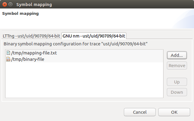
Simply click the Add... button to add one or multiple mapping files. The mapping file could be one of two options:
 : a binary that was used for taking the trace.
 : a file generated from the binary using
nm myprogram > mapping.txt. Select the
mapping.txt file that was just created. If you are dealing with C++ executables, you may want to use
nm --demangle instead to get readable function names.
: a file generated from the binary using
nm myprogram > mapping.txt. Select the
mapping.txt file that was just created. If you are dealing with C++ executables, you may want to use
nm --demangle instead to get readable function names.
The view should now update to display the function names instead. Make sure the binary used for taking the trace is the one used for this step too (otherwise, there is a good chance of the addresses not being the same).
Lastly, the basic symbol provider introduces the notion of priorities between the mapping files. The resolved symbols from the file at the top of the list will have a higher priority than the files listed below. The files can be moved using the Up and Down buttons.
See Control Flow View's Using the mouse , Using the keyboard and Zoom region .
See Control Flow View's Marker Axis .
This is an aggregate view of the function calls from the Flame Chart View. This shows a bird's eye view of what are the main time sinks in the traced applications. Each entry in the Flame Graph represents an aggregation of all the calls to a function in a certain depth of the call stack having the same caller. So, functions in the Flame Graph are aggregated by depth and caller. This enables the user to find the most executed code path easily.
The function name is visible on each Flame graph event if the size permits. Each box in the Flame Graph has the same color as the box representing the same function in the Flame Chart.
To open this view, select a trace, expand it in the Project Explorer, then expand the Call Graph Analysis (the trace must be loaded) and open the Flame Graph. It's also possible to go in Window -> Show View -> Tracing then select Flame Graph in the list.

To use the Flame graph, one can navigate it and find which function is consuming the most self-time. This can be seen as a large plateau. Then the entry can be inspected. At this point, the worst offender in terms of CPU usage will be highlighted, however, it is not a single call to investigate, but rather the aggregation of all the calls. Right mouse-clicking on that entry will open a context sensitive menu. Selecting Go to minimum or Go to maximum will take the user to the minimum or maximum recorded times in the trace. This is interesting to compare and contrast the two.
Hovering over a function will show a tooltip with the statistics on a per-function basis. One can see the total and self times ( worst-case, best-case, average, total time, standard deviation, number of calls) for that function.
If one wishes to explore at a medium detail level between the "classic" flame graph view and the call stack view, a per-thread flame graph view is available by selecting the coarser menu and clicking on Content Presentation then Per-thread. To return to the default mode, return to that menu and click on Aggregate Threads.
Observing the time spent in each function can show where most of the time is spent and where one could optimize. An example in the image above: one can see that mp_sort is a recursive sort function, it takes approximately 40% of the execution time of the program. That means that perfectly parallelizing it can yield a gain of 20% for 2 threads, 33% for 3 and so forth. Looking at the function print_current_files, it takes about 30% of the time, and it has a child print_many_per_line that has a large self time (above 10%). This could be another area that can be targeted for optimization. Knowing this in advance helps developers know where to aim their efforts.
It is recommended to have a kernel trace as well as a user space trace in an experiment while using the Flame Graph as it will show what is causing the largest delays. When using the Flame Graph together with a call stack and a kernel trace, an example work flow would be to find the worst offender in terms of time taken for a function that seems to be taking too long. Then, using the context menu Go to maximum, one can navigate to the maximum duration and see if the OS is, for example, preempting the function for too long, or if the issue is in the code being executed.
This displays the descriptive statistics of the 'wall time' durations of given functions. It gives an overview of how often a function is called, how much total time it took, its mean duration as well as its maximum, minimum times and the standard deviation.
If a time range is selected it will display the local statistics too.
This analysis is available if the Flame Graph is available.
When the mouse cursor is over entries (left pane):
The following keyboard shortcuts are available:

|
Sort by thread name | Sort the threads by thread name. Clicking the icon a second time will sort the threads by name in reverse order and change the icon to

|

|
Sort by thread id | Sort the threads by thread ID. Clicking the icon a second time will sort the threads by ID in reverse order and change the icon to
 . .
|
See Flame Chart View's Importing a binary or function name mapping file (for LTTng-UST <2.8 traces) .
The Function Duration Density view shows the function duration of function displayed by duration for the current active time window range. This is useful to find global outliers.

Using the right mouse button to drag horizontally it will update the table and graph to show only the density for the selected durations. Durations outside the selection range will be filtered out. Using the toolbar button
 the zoom range will be reset.
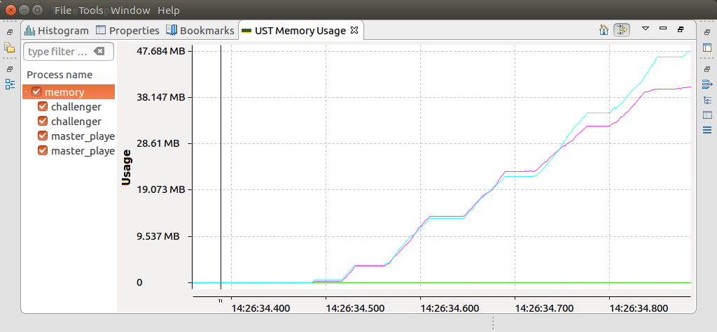
The Memory Usage view allows the user to visualize the active memory usage per thread over time, if the application and trace provide this information.
The view shows the memory consumption for the currently selected trace.
The time chart plots heap memory usage graphically over time. There is one line per process, unassigned memory usage is mapped to "Other". Processes can be checked and unchecked in the tree on the left hand side.
The filter button:
 can be used to show only the active threads in the tree viewer. By default only the threads which have had memory usage variations in the visible time range will be shown, clicking the button will reveal all the threads.
In this implementation, the user needs to trace while hooking the liblttng-ust-libc-wrapper by running LD_PRELOAD=liblttng-ust-libc-wrapper.so <exename>. This will add tracepoints to memory allocation and freeing to the heap, NOT shared memory or stack usage. If the contexts vtid and procname are enabled, then the view will associate the heap usage to processes. As detailed earlier, to enable the contexts, see the Adding Contexts to Channels and Events of a Domain section. Or if using the command-line:
lttng add-context -u -t vtid -t procname
If thread information is available the view will look like this:
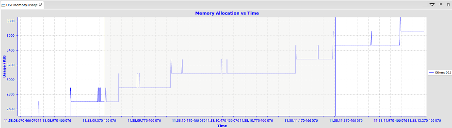
If thread information is not available it will look like this:
The time axis is aligned with other views that support automatic time axis alignment (see Automatic Time Axis Alignment).
The time range can be fully zoomed out by double-clicking the time axis or the home button.
Please note this view will not show shared memory or stack memory usage.
For navigation, see CPU Usage view's Using the mouse , Using the keyboard and Zoom region .
The view toolbar, located at the top right of the view, has shortcut buttons to perform common actions.
For details about the see CPU Usage view's Toolbar .
The Memory Usage View view menu, located at the top right of the view, has shortcut buttons to perform common actions:
| New Memory Usage view | Spawn a new Memory Usage view. The new view can be pinned to a new instance of the current trace, pinned to any opened trace, or unpinned. |
| Export... | Opens a file menu to choose a file name to export the current time chart to a PNG image. |
| Align Views | Disable and enable the automatic time axis alignment of time-based views. Disabling the alignment in this view will disable this feature across all the views because it's a workspace preference. |
Please note this view will not show shared memory or stack memory usage.
Starting with LTTng 2.8, the tracer can now provide enough information to associate trace events with their location in the original source code.
To make use of this feature, first make sure your binaries are compiled with debug information (-g), so that the instruction pointers can be mapped to source code locations. This lookup is made using the addr2line and nm command-line utilities, which need to be installed and on the $PATH of the system running Trace Compass. addr2line and nm are available in most Linux distributions, Mac OS X, Windows using Cygwin and others.
The following trace events need to be present in the trace:
as well as the following contexts:
For ease of use, you can simply enable all the UST events when setting up your session:
 lttng enable-event -u -a
 lttng add-context -u -t vpid -t ip
Note that you can also create and configure your session using the Control View.
If you want to track source locations in shared libraries loaded by the application, you also need to enable the "lttng_ust_dl:*" events, as well as preload the UST library providing them when running your program:
LD_PRELOAD=/path/to/liblttng-ust-dl.so ./myprogram
If all the required information is present, then the Source Location column of the Event Table should be populated accordingly, and the Open Source Code action should be available. Refer to the section Event Source Lookup for more details.
The Binary Location information should be present even if the original binaries are not available, since it only makes use of information found in the trace. A + denotes a relative address (i.e. an offset within the object itself), whereas a @ denotes an absolute address, for non-position-independent objects.
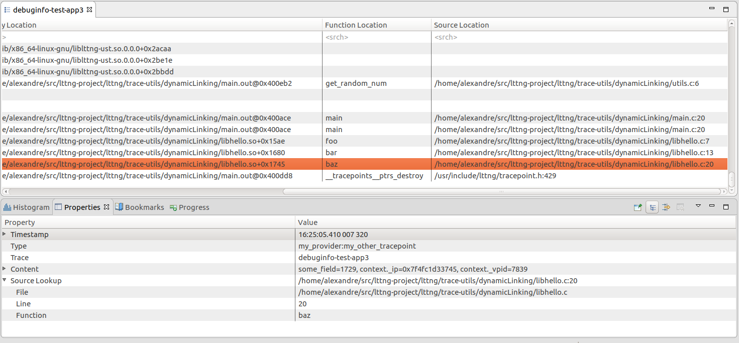
Example of a trace with debug info and corresponding Source Lookup information, showing a tracepoint originating from a shared library
To resolve addresses to function names and source code locations, the analysis makes use of the binary files (executables or shared libraries) present on the system. By default, it will look for the file paths as they are found in the trace, which means that it should work out-of-the-box if the trace was taken on the same machine that Trace Compass is running.
It is possible to configure a root directory that will be used as a prefix for all file path resolutions. The button to open the configuration dialog is called Configure how addresses are mapped to function names and is currently located in the Flame Chart View. Note that the Call Stack View will also make use of this configuration to resolve its function names.
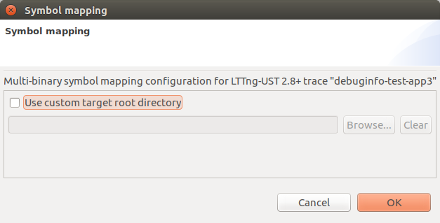
The symbol configuration dialog for LTTng-UST 2.8+ traces
This can be useful if a trace was taken on a remote target, and an image of that target is available locally.
If a binary file is being traced on a target, the paths in the trace will refer to the paths on the target. For example, if they are:
and an image of that target is copied locally on the system at /home/user/project/image, which means the binaries above end up at:
Then selecting the /home/user/project/image directory in the configuration dialog above will allow Trace Compass to read the debug symbols correctly.
Note that this path prefix will apply to both binary file and source file locations, which may or may not be desirable.
|
|

|
|
| LTTng Kernel Analysis | Trace synchronization |