

| LTTng Kernel Analysis | ||
|---|---|---|
|
|
|
|
| LTTng Tracer Control | LTTng-UST Analyses | |
Historically, LTTng was developed to trace the Linux kernel and, over time, a number of kernel-oriented analysis views were developed and organized in a perspective.
This section presents a description of the OS Tracing Overview perspective and the LTTng Kernel perspective.
The OS Tracing Overview perspective groups the following views:
The perspective can be opened from the Eclipse Open Perspective dialog ( Window > Open Perspective... > Other).
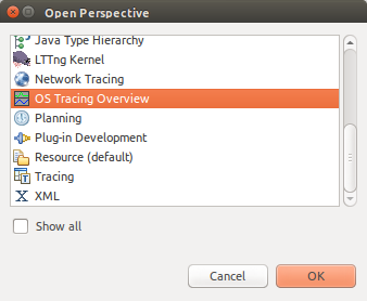
This perspective is intended to be used to locate performance issues by observing resource usage.
The perspective can show times resource usage is anomalous. This can help locating the causes of system slowdowns in throughput or response time.
An example can be program that is doing a lot of processing then slows down due to a database access. The user will see a dip in CPU usage and maybe a slight rise in I/O access. The user should consider both spike and slums to be an indication of an area worth investigating.
Once a performance issue has been localized, it can be further investigated with the #LTTng kernel Perspective.
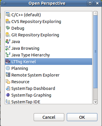
The LTTng Kernel perspective is built upon the Tracing Perspective, re-organizes them slightly and adds the following views:
The perspective can be opened from the Eclipse Open Perspective dialog ( Window > Open Perspective... > Other).
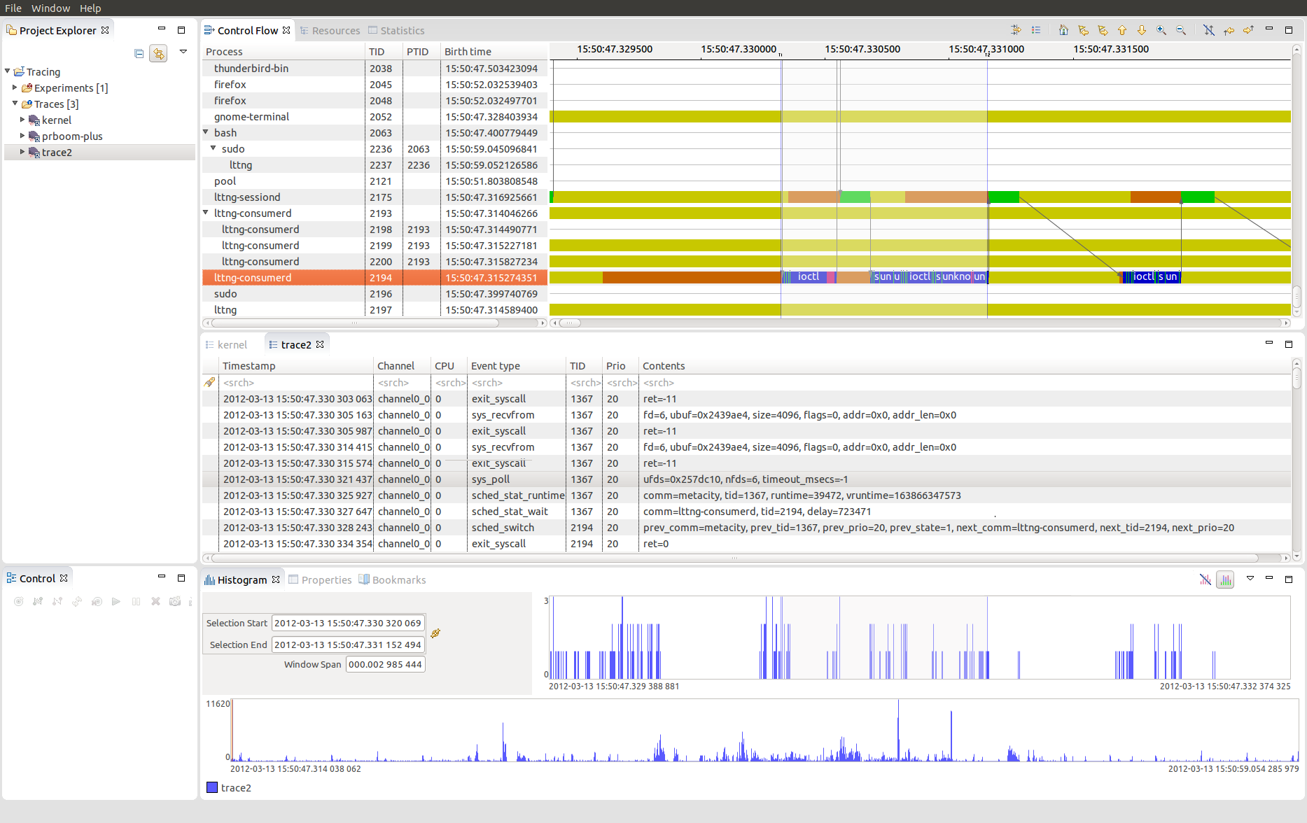
The Control Flow view is a LTTng-specific view that shows per-process events graphically. The Linux Kernel Analysis is executed the first time a LTTng Kernel is opened. After opening the trace, the element Control Flow is added under the Linux Kernel Analysis tree element in the Project Explorer. To open the view, double-click the Control Flow tree element.
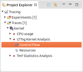
Alternatively, select Control Flow under LTTng within the Show View window ( Window -> Show View -> Other...):
You should get something like this:
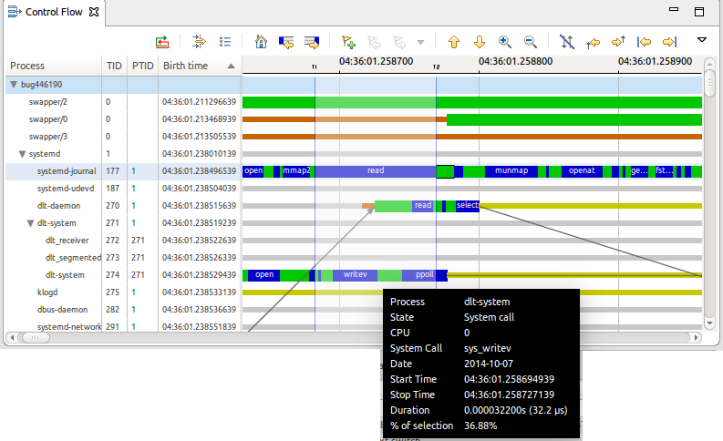
The view is divided into the following important sections: process tree and information, control flow and the toolbar. The time axis is aligned with other views that support automatic time axis alignment (see Automatic Time Axis Alignment).
The following sections provide detailed information for each part of the Control Flow View.
Processes are organized as a tree within this view. This way, child and parent processes are easy to identify.
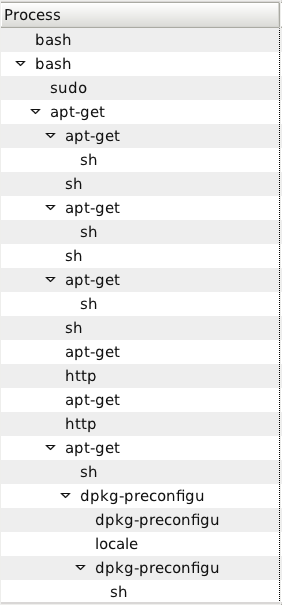
The layout is based on the states computed from the trace events.
A given process may be shown at different places within the tree since the nodes are unique (TID, birth time) couples. This means that if process B of parent A dies, you'll still see it in the tree. If process A forks process B again, it will be shown as a different node since it won't have the same birth time (and probably not the same TID). This has the advantage that the tree, once loaded, never changes: horizontal scrolling within the control flow remains possible.
The TID column shows the process node's thread ID and the PTID column shows its parent thread ID (nothing is shown if the process has no parent).
It is possible to sort the columns of the tree by clicking on the column header. Subsequent clicking will change the sort order. The hierarchy, i.e. the parent-child relationship is kept. When opening a trace for the first time, the processes are sorted by birth time. The sort order and column will be preserved when switching between open traces. Note that when opening an experiment the processes will be sorted within each trace.
This part of the Control Flow View is probably the most interesting one. Using the mouse, you can navigate through the trace (go left, right) and zoom on a specific region to inspect its details.
The colored bars you see represent states for the associated process node. When a process state changes in time, so does the color. For state SYSCALL the name of the system call is displayed in the state bar. States colors legend is available through a toolbar button:
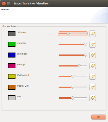
The style can be updated in the legend.
This dark yellow is what you'll see most of the time since scheduling puts processes on hold while others run.
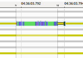
The vertical blue line with T1 above it is the current selection indicator. When a time range is selected, the region between the begin and end time of the selection will be shaded and two lines with T1 and T2 above will be displayed. The time stamps corresponding to T1, T2 and their delta are shown in the status line when the mouse is hovering over the control flow.
Arrows can be displayed that follow the execution of each CPU across processes. The arrows indicate when the scheduler switches from one process to another for a given CPU. The CPU being followed is indicated on the state tooltip. When the scheduler switches to and from the idle process, the arrow skips to the next process which executes on the CPU after the idle process. Note that an appropriate zoom level is required for all arrows to be displayed.
The display of arrows is optional and can be toggled using the Hide Arrows toolbar button. It is also possible to follow a CPU's execution across state changes and the scheduler's process switching using the Follow CPU Forward/Backward toolbar buttons.
The following mouse actions are available:
When the current time indicator is changed (when clicking in the states flow), all the other views are synchronized. For example, the Events Editor will show the event matching the current time indicator. The reverse behaviour is also implemented: selecting an event within the Events View will update the Control Flow View current time indicator.
The following keyboard shortcuts are available:
WASD Navigation
Use WASD Navigation in conjunction with the mouse, where one hand changes the mouse position and the other hand uses the keyboard shortcuts to zoom or scroll.
When the mouse cursor is over entries (left pane):
Please note that the behavior of some shortcuts can slightly differ based on the operating system.
When the selection indicators are changed, all the other views are synchronized. For example, the Events Editor will show the event matching the current time indicator. The reverse behaviour is also implemented: selecting an event within the Events View will update the Control Flow View current time indicator.
You'll notice small dots over the colored bars at some places:
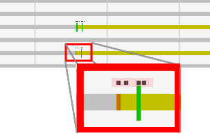
Those dots mean the underlying region is incomplete: there's not enough pixels to view all the events. In other words, you have to zoom in.
When zooming in, small dots start to disappear:
When no dots are left, you are viewing all the events and states within that region.
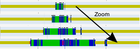
To zoom in on a specific region, right-click and drag in order to draw a time range:
The states flow horizontal space will only show the selected region.
Hover the cursor over a colored bar and a tooltip will pop up:
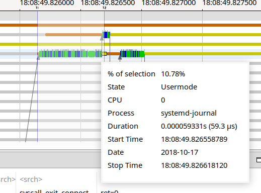
The tooltip indicates:
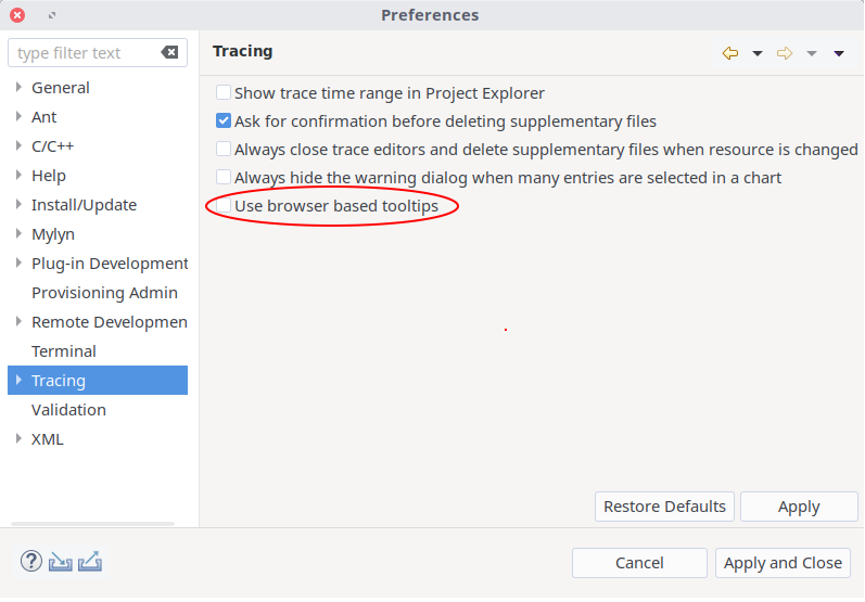
A browser based tooltip is available that allows users to use hyperlink navigation or to copy text. To enable the feature select
Window-> Preferences-> Tracing then checking Use browser based tooltips. It is known to be unstable on older platforms, if this instability is encountered, please submit your bug here: https://bugs.eclipse.org/bugs/show_bug.cgi?id=547563
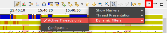
Dynamic filters are filters that are processed and applied each time the control flow view visible time range changes.
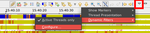
The dynamics filters can be rapidly toggled in their view sub menu.
The dynamics filters can be fine tuned in the configuration dialog.
Note: Dynamic filters can induce performance degradation.
The Show Active Threads Only filter allow a user to increase the signal to noise ratio by filtering out all inactive threads.
A thread is considered inactive when it is in the following state:
A user can fine tune this filter by providing ranges of CPUs allowing the filter to only show active thread running on the specified CPUs.

The Control Flow View toolbar, located at the top right of the view, has shortcut buttons to perform common actions:
|
|
Hide Empty Rows | If button is checked, it hides rows that are empty, else they are shown. This setting will be preserved when switching between open traces. |

|
Show View Filter | Opens the process filter dialog. Filter settings will be preserved when switching between open traces. |

|
Show Legend | Displays the states legend. |

|
Optimize | "Optimize" the row order of the control flow view. This groups the threads by minimizing the distance in the graph of transitions by CPU for a given time range. The scheduler will often keep tightly coupled threads on the same CPU to preserve data locality. An interesting side effect of this is that threads communicating together in that time range will be moved closer together when pressing the button. The button moves the rows only when pressed. When the time range is moved, the optimization action can be re-applied. |

|
Reset the Time Scale to Default | Resets the zoom window to the full range. |

|
Select Previous State Change | Selects the previous state for the selected process. Pressing the Shift key at the same time will update the selection end time of the current selection range. |

|
Select Next State Change | Selects the next state for the selected process. Pressing the Shift key at the same time will update the selection end time of the current selection range. |

|
Add Bookmark... | Adds a bookmark at the current selection range. A bookmark is a user-defined interval marker. The Add Bookmark dialog is opened where the user can enter a description and choose the highlighting color and alpha (transparency) value. This button is replaced by the Remove Bookmark button if the current selection range corresponds to an existing bookmark. The bookmarks can also be managed in the Bookmark View. |

|
Remove Bookmark | Removes the bookmark at the current selection range. This button replaces the Add Bookmark when the current selection range corresponds to an existing bookmark. |

|
Previous Marker | Selects the previous active marker. Pressing the Shift key at the same time will update the selection end time of the current selection range. |

|
Next Marker | Selects the next active marker. Pressing the Shift key at the same time will update the selection end time of the current selection range. Clicking the button drop-down arrow will open a menu where marker categories can be made active or inactive for navigation. To toggle the display of a marker category, use the View Menu instead. |

|
Select Previous Process | Selects the previous process. |

|
Select Next Process | Selects the next process. |

|
Zoom In | Zooms in on the selection by 50%. |

|
Zoom Out | Zooms out on the selection by 50%. |

|
Hide Arrows | Toggles the display of arrows on or off. |
|
|
Follow CPU Backward | Selects the previous state following CPU execution across processes. Pressing the Shift key at the same time will update the selection end time of the current selection range. |
|
|
Follow CPU Forward | Selects the next state following CPU execution across processes. Pressing the Shift key at the same time will update the selection end time of the current selection range. |

|
Go to previous event of the selected thread | Move to the closest previous event belonging to the selected thread. This action looks through all trace events, unlike the Select Previous State Change action which only stops at state changes. |

|
Go to next event of the selected thread | Move to the closest following event belonging to the selected thread. This action looks through all trace events, unlike the Select Next State Change action which only stops at state changes. |


|
Pin/Unpin View | Pin or unpin the view. A pinned view is frozen with the trace selected at the time of pinning. When the unpin button is clicked the view synchronizes back to the active trace. The button's drop down menu can be used to quickly pin the view to any of the opened traces. |
View Menu
| New Control Flow view | Spawn a new Control Flow view. The new view can be pinned to a new instance of the current trace, pinned to any opened trace, or unpinned. |
| Export... | Opens a file menu to choose a file name to export the current time graph to a PNG image. |
| Align Views | Disable and enable the automatic time axis alignment of time-based views. Disabling the alignment in this view will disable this feature across all the views because it's a workspace preference. |
| Show Gridlines | Toggles visibility of Horizontal and Vertical gridlines. |
| Show Labels | Toggles visibility of labels. |
| Show Markers | A marker highlights a time interval. A marker can be used for instance to indicate a time range where lost events occurred or to bookmark an interesting interval for future reference. Selecting a category name will toggle the visibility of markers of that category. |
| Marker Set | The user can select from one of the configured market sets, or choose None to use no marker set. The setting applies to all views that support marker sets. The marker set configuration can be edited by selecting the Edit... menu item (see Marker Set Configuration XML Format). After saving the changes in the opened editor, the marker set should then be re-selected to update the view. |
| Hide Empty Rows | If button is checked, it hides rows that are empty, else they are shown. This setting will be preserved when switching between open traces. |
| Thread Presentation | Select the threads layout. Two layouts are available. Flat layout lists the threads in a flat list per trace. Hierarchical layout shows the threads in a parent-child tree per trace. |
| Dynamic Filters | Select and configure the Dynamic Filters to be applied. |
The marker axis is visible only when at least one marker category with markers for the current trace is shown.
The marker axis displays one row per marker category. Each marker's time range and/or label (if applicable) are drawn on the marker axis.
Clicking on any marker's time range or label will set the current time selection to the marker's time or time range. Shift-clicking will extend the current time selection to include the marker's time or time range.
Clicking on the "X" icon to the left of the marker category name will hide this marker category from the time graph. It can be shown again using the corresponding Show Markers menu item in the view menu.
The marker axis can be collapsed and expanded by clicking on the icon at the top left of the marker axis. The marker axis can be completely removed by hiding all available marker categories.
This view is specific to LTTng kernel traces. The Linux Kernel Analysis is executed the first time a LTTng Kernel is opened. After opening the trace, the element Resources is added under the Linux Kernel Analysis tree element of the Project Explorer. To open the view, double-click the Resources tree element.
Alternatively, go in Window -> Show View -> Other... and select LTTng/Resources in the list.

This view shows the state of system resources i.e. if changes occurred during the trace either on CPUs, IRQs or soft IRQs, it will appear in this view. The left side of the view present a list of resources that are affected by at least one event of the trace. The right side illustrate the state in which each resource is at some point in time. For state USERMODE it also prints the process name in the state bar. For state SYSCALL the name of the system call is displayed in the state region.
When an IRQ is handled by a CPU, its states are shown under the corresponding CPU entry. Similarly, the CPU that was handling an IRQ is shown under the handled IRQ. Therefore, the trace can be visualized from a CPU point of view or from an IRQ point of view.
Just like other views, according to which trace points and system calls are activated, the content of this view may change from one trace to another.
The time axis is aligned with other views that support automatic time axis alignment (see Automatic Time Axis Alignment).
Each state are represented by one color so it is faster to say what is happening.

The style can be updated in the legend.
To go through the state of a resource, you first have to select the resource and the timestamp that interest you. For the latter, you can pick some time before the interesting part of the trace.

Then, by selecting Next Event, it will show the next state transition and the event that occurred at this time.

This view is also synchronized with the others: Histogram View, Events Editor, Control Flow View, etc.
It is possible to follow a CPU by right-clicking on its entry in the view, then selecting Follow CPU X where X is the number of the CPU. Following a CPU will filter the CPU Usage View to display only usage for the selected CPU. To unfollow a CPU, one needs to right-click on any CPU entry and select Unfollow CPU.
It is possible to follow a thread by right-clicking on a thread time event in a CPU thread status line, then selecting Follow TID X where X is the TID number of the thread to follow. Following a thread will display a red box around all the time events belonging to that specific thread. To unfollow a thread, one needs to right-click on any thread time event and select Unfollow.

See Control Flow View's Using the mouse , Using the keyboard and Zoom region .
See Control Flow View's Incomplete regions .
The Resources View toolbar, located at the top right of the view, has shortcut buttons to perform common actions:
|
|
Hide Empty Rows | If button is checked, it hides rows that are empty, else they are shown. This setting will be preserved when switching between open traces. |
|
|
Show View Filter | Opens the resources filter dialog. Filter settings will be preserved when switching between open traces. |
|
|
Show Legend | Displays the states legend. |
|
|
Reset the Time Scale to Default | Resets the zoom window to the full range. |
|
|
Select Previous State Change | Selects the previous state for the selected resource. Pressing the Shift key at the same time will update the selection end time of the current selection range. |
|
|
Select Next State Change | Selects the next state for the selected resource. Pressing the Shift key at the same time will update the selection end time of the current selection range. |
|
|
Add Bookmark... | Adds a bookmark at the current selection range. A bookmark is a user-defined interval marker. The Add Bookmark dialog is opened where the user can enter a description and choose the highlighting color and alpha (transparency) value. This button is replaced by the Remove Bookmark button if the current selection range corresponds to an existing bookmark. The bookmarks can also be managed in the Bookmark View. |
|
|
Remove Bookmark | Removes the bookmark at the current selection range. This button replaces the Add Bookmark when the current selection range corresponds to an existing bookmark. |
|
|
Previous Marker | Selects the previous active marker. Pressing the Shift key at the same time will update the selection end time of the current selection range. |
|
|
Next Marker | Selects the next active marker. Pressing the Shift key at the same time will update the selection end time of the current selection range. Clicking the button drop-down arrow will open a menu where marker categories can be made active or inactive for navigation. |
|
|
Select Previous Resource | Selects the previous resource |
|
|
Select Next Resource | Selects the next resource |
|
|
Zoom In | Zooms in on the selection by 50%. |
|
|
Zoom Out | Zooms out on the selection by 50%. |
|
|
Pin/Unpin View | Pin or unpin the view. A pinned view is frozen with the trace selected at the time of pinning. When the unpin button is clicked the view synchronizes back to the active trace. The button's drop down menu can be used to quickly pin the view to any of the opened traces. |
View Menu
| New Resources view | Spawn a new Resources view. The new view can be pinned to a new instance of the current trace, pinned to any opened trace, or unpinned. |
| Export... | Opens a file menu to choose a file name to export the current time graph to a PNG image. |
| Align Views | Disable and enable the automatic time axis alignment of time-based views. Disabling the alignment in this view will disable this feature across all the views because it's a workspace preference. |
| Show Gridlines | Toggles visibility of Horizontal and Vertical gridlines. |
| Show Labels | Toggles visibility of labels. |
| Show Markers | A marker highlights a time interval. A marker can be used for instance to indicate a time range where lost events occurred or to bookmark an interesting interval for future reference. Selecting a category name will toggle the visibility of markers of that category. |
| Marker Set | The user can select from one of the configured market sets, or choose None to use no marker set. The setting applies to all views that support marker sets. The marker set configuration can be edited by selecting the Edit... menu item (see Marker Set Configuration XML Format). After saving the changes in the opened editor, the marker set should then be re-selected to update the view. |
| Hide Empty Rows | If button is checked, it hides rows that are empty, else they are shown. This setting will be preserved when switching between open traces. |
See Control Flow View's Marker Axis .
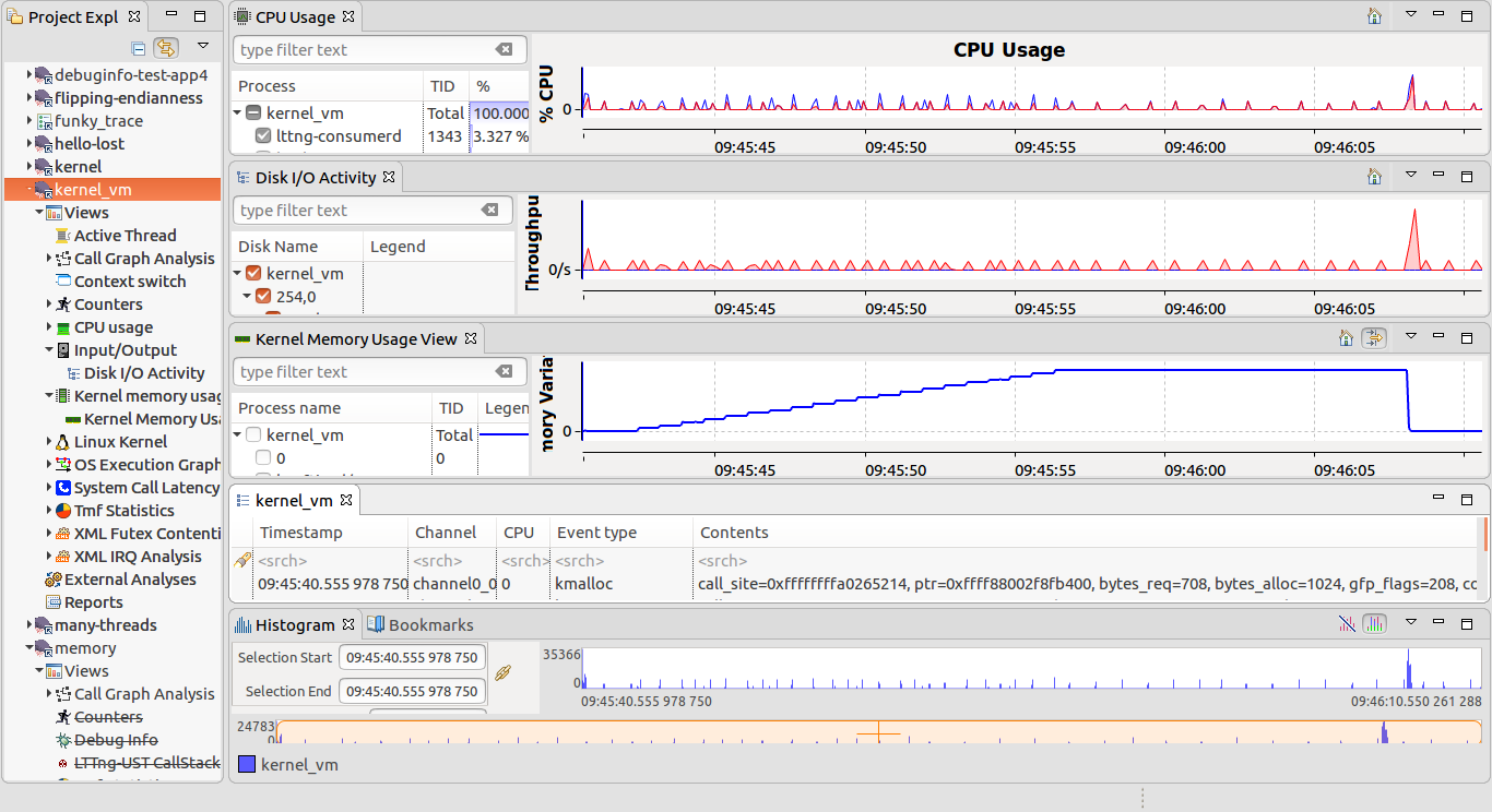
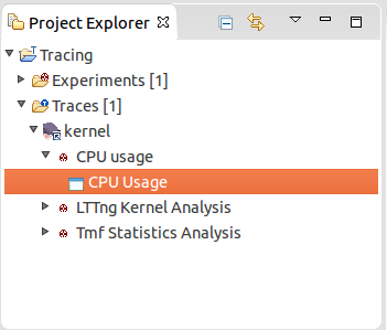
The CPU Usage analysis and view is specific to LTTng Kernel traces. The CPU usage is derived from a kernel trace as long as the sched_switch event was enabled during the collection of the trace. This analysis is executed the first time that the CPU Usage view is opened after opening the trace. To open the view, double-click on the CPU Usage tree element under the Linux Kernel Analysis tree element of the Project Explorer.
Now, the CPU Usage view will show:

The view is divided into the following important sections: Process Information and the CPU Usage Chart. The time axis is aligned with other views that support automatic time axis alignment (see Automatic Time Axis Alignment).
The Process Information is displayed on the left side of the view and shows all threads that were executing on all available CPUs in the current time range. For each process, it shows in different columns the thread ID (TID), process name (Process), the average (%) execution time and the actual execution time (Time) during the current time range. It shows all threads that were executing on the CPUs in the current time range.
The CPU Usage Chart on the right side of the view, plots the total time spent on all CPUs of all processes and the time of the selected process.
Hover the cursor over a line of the chart and a tooltip will pop up with the following information:
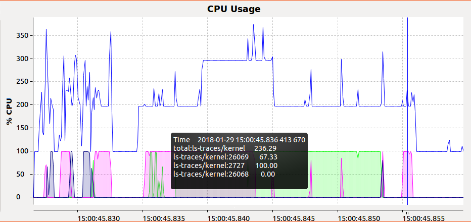
The CPU Usage chart is usable with the mouse. The following actions are set:
The following keyboard shortcuts are available, when the mouse cursor is over the graph (right pane):
WASD Navigation
Use WASD Navigation in conjunction with the mouse, where one hand changes the mouse position and the other hand uses the keyboard shortcuts to zoom or scroll.
The view toolbar, located at the top right of the view, has shortcut buttons to perform common actions:
|
|
Reset the Time Scale to Default | Resets the zoom window to the full range. |
|
|
Zoom In | Zooms in on the selection by 50%. |
|
|
Zoom Out | Zooms out on the selection by 50%. |
|
|
Pin/Unpin View | Pin or unpin the view. A pinned view is frozen with the trace selected at the time of pinning. When the unpin button is clicked the view synchronizes back to the active trace. The button's drop down menu can be used to quickly pin the view to any of the opened traces. |
The CPU Usage View view menu, located at the top right of the view, has shortcut buttons to perform common actions:
| New CPU Usage view | Spawn a new CPU Usage view. The new view can be pinned to a new instance of the current trace, pinned to any opened trace, or unpinned. |
| Export... | Opens a file menu to choose a file name to export the current time chart to a PNG image. |
| Align Views | Disable and enable the automatic time axis alignment of time-based views. Disabling the alignment in this view will disable this feature across all the views because it's a workspace preference. |
Follow a CPU will filter the CPU Usage View and will display only usage for the followed CPU.
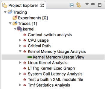
The Kernel Memory Usage and view is specific to kernel traces. To open the view, double-click on the Kernel Memory Usage Analysis tree element under the Kernel tree element of the Project Explorer.
Now, the Kernel memory usage view will show:

Where:
The view is divided into the following important sections: Process Information and the Relative Kernel Memory Usage. The time axis is aligned with other views that support automatic time axis alignment (see Automatic Time Axis Alignment).
The filter button:
can be used to show only the active threads in the tree viewer. By default only the threads which have had memory usage variations in the visible time range will be shown, clicking the button will reveal all the threads. Threads can be filtered by checking and unchecking them in the left hand side tree.
The time range can be set to fully zoomed out by double-clicking the time axis or the home button.
The Process Information is displayed on the left side of the view and shows all threads that were executing on all available CPUs in the current time range. For each process, it shows in different columns the thread ID (TID) and the process name (Process).
For navigation, see CPU Usage view's Using the mouse , Using the keyboard and Zoom region .
The view toolbar, located at the top right of the view, has shortcut buttons to perform common actions:
|
|
Filter active threads | Show only active threads |
For other toolbar buttons, see CPU Usage view's Toolbar .
The Memory Usage View view menu, located at the top right of the view, has shortcut buttons to perform common actions:
| New Memory Usage view | Spawn a new Memory Usage view. The new view can be pinned to a new instance of the current trace, pinned to any opened trace, or unpinned. |
| Export... | Opens a file menu to choose a file name to export the current time chart to a PNG image. |
| Align Views | Disable and enable the automatic time axis alignment of time-based views. Disabling the alignment in this view will disable this feature across all the views because it's a workspace preference. |
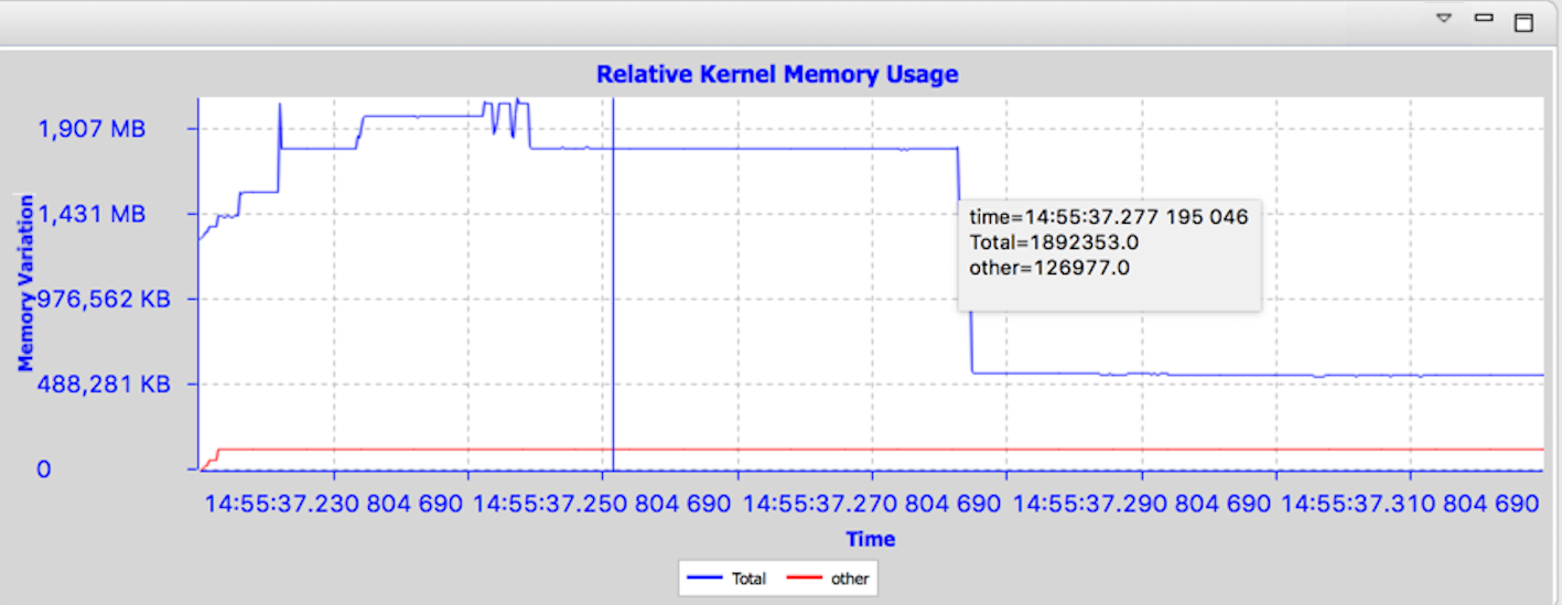
The Relative Kernel Memory Chart on the right side of the view plots the relative amount of memory that was allocated and deallocated during that period of time.
For navigation, see CPU Usage view's Using the mouse , Using the keyboard and Zoom region .
Hover the cursor over a line of the chart and a tooltip will pop up with the following information:
TraceCompass can recover wait causes of local and distributed processes using operating system events. The analysis highlights the tasks and devices causing wait. Wait cause recovery is recursive, comprise all tasks running on the system and works across computers using packet trace synchronization.
The analysis details are available in the paper Wait analysis of distributed systems using kernel tracing.
The analysis requires a Linux kernel trace. Additional instrumentation may be required for specific kernel version and for distributed tracing. This instrumentation is available in LTTng modules addons on GitHub.
The required events are:
To analyze a distributed program, all computers involved in the processing must be traced simultaneously. The LTTng Tracer Control of TraceCompass can trace a remote computer, but controlling simultaneous tracing is not supported at the moment, meaning that all sessions must be started separately and interactively. TraceCompass will support this feature in the future. For now, it is suggested to use lttng-cluster command line tool to control simultaneous tracing sessions on multiple computers. This tool is based on Fabric and uses SSH to start the tracing sessions, execute a workload, stop the sessions and gather traces on the local computer. For more information, refer to the lttng-cluster documentation.
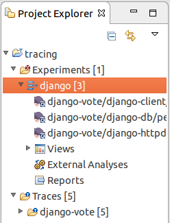
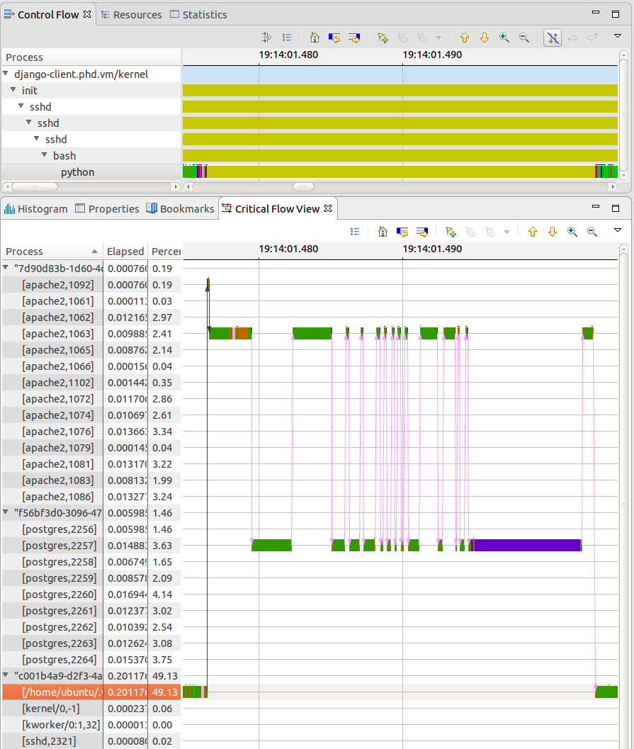
We use the Django trace as an example to demonstrate the wait analysis. Django is a popular Web framework. The application is the Django Poll app tutorial. The traces were recorded on three computers, namely the client (implemented with Python Mechanize), the Web server (Apache with WSGI) and the database server (PostgreSQL). The client simulates a vote in the poll.
To open all three traces simultaneously, we first create an experiment containing these traces and then synchronize the traces, such that they have a common time base. Then, the analysis is done by selecting a task in the Control Flow View. The result is displayed in the Critical Flow View, which works like the Control Flow View. The steps to load the Django example follows.
 displays the colors associated with the processes states.
TraceCompass can analyse disk input/output through the read/write system calls to get the read/write per processes, but also with the disk request events, to get the actual reads and writes to disk.
The following tracepoints should be enabled to get the disk read/write data. Also, enabling syscalls will allow to match the reads and writes per processes.
   # sudo lttng list -k
   Kernel events:
   -------------
     ...
     block_rq_complete (loglevel: TRACE_EMERG (0)) (type: tracepoint)
     block_rq_insert (loglevel: TRACE_EMERG (0)) (type: tracepoint)
     block_rq_issue (loglevel: TRACE_EMERG (0)) (type: tracepoint) # on the guest
     block_bio_frontmerge (loglevel: TRACE_EMERG (0)) (type: tracepoint) # on the guest
     ...
For full disk request tracking, some extra tracepoints are necessary. They are not required for the I/O analysis, but make the analysis more complete. Here is the procedure to get those tracepoints that are not yet part of the mainline kernel.
   # git clone https://github.com/giraldeau/lttng-modules.git
   # cd lttng-modules
Checkout the addons branch, compile and install lttng-modules as per the lttng-modules documentation.
   # git checkout addons
   # make
   # sudo make modules_install
   # sudo depmod -a
The lttng addons modules must be inserted manually for the extra tracepoints to be available:
   # sudo modprobe lttng-addons
   # sudo modprobe lttng-elv
And enable the following tracepoint
addons_elv_merge_requests
The following views are available for input/output analyses:
A time aligned XY chart of the read and write speed for the different disks on the system. This view is useful to see where there was more activity on the disks and whether it was mostly reads or writes.
Disk reads and writes can be selected in the tree on the left hand side.
The time range can be reset by double-clicking the time axis or by clicking the reset button.
For navigation, see CPU Usage view's Using the mouse , Using the keyboard and Zoom region .
The view toolbar, located at the top right of the view, has shortcut buttons to perform common actions.
For details about the see CPU Usage view's Toolbar .
The Disk I/O View view menu, located at the top right of the view, has shortcut buttons to perform common actions:
| New Disk I/O Activity view | Spawn a new Disk I/O Activity view. The new view can be pinned to a new instance of the current trace, pinned to any opened trace, or unpinned. |
| Export... | Opens a file menu to choose a file name to export the current time chart to a PNG image. |
| Align Views | Disable and enable the automatic time axis alignment of time-based views. Disabling the alignment in this view will disable this feature across all the views because it's a workspace preference. |
The System Call Latency Analysis measures the system call latency between system call entry and exit per type of system call. The durations are visualized using the Latency views. For more information about the Latency views see chapter Latency Analyses.
The Futex Contention Latency Analysis measures the futexes contention latency between futex entry and exit event for a thread. The durations are visualized using the Latency views. For more information about the Latency views see chapter Latency Analyses.
The following views are also available for the Futex Contention Latency Analysis:
A timegraph view of the waiters by futex uaddr. This view is useful to see which threads are waiting on a specific futex and understand blocked threads.

A timegraph view of the futex wait/lock and wake/unlock scenarios (from futex entry to futex exit). This view is useful to suss up the general level of contention in a given trace. It highlights futex lifespans.

The Latency analysis for IRQ handlers measures the latency between the IRQ handlers entry and exit events. The durations are visualized using the Latency views. For more information about the Latency views see chapter Latency Analyses.
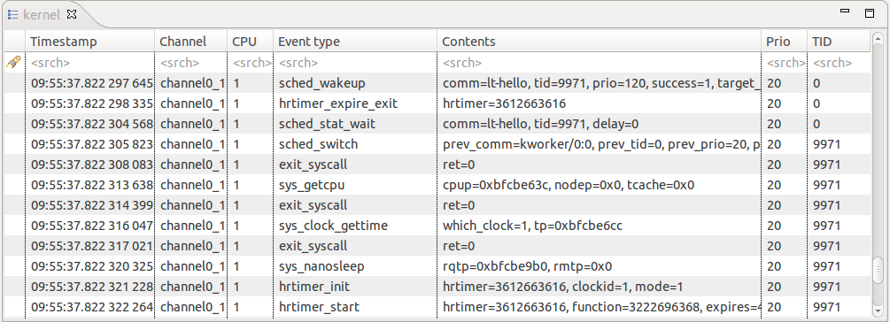
The LTTng Kernel Events editor is the plain TMF Events Editor, except that it provides its own specialized viewer to replace the standard one. In short, it has exactly the same behaviour but the layout is slightly different:
The Scheduler wake up/Scheduler switch Latency Analysis measures the latency between the sched_wakeup (scheduler wake up) and sched_switch (scheduler switch) event. In layman's terms, the analysis measures the time from the moment a process/thread wakes up until it is switched onto the CPU. The durations are visualized using the Latency views. For more information about the Latency views see chapter Latency Analyses.
Besides the typical latency views, the analysis also provides a Priority/Thread name Statistics view. The view groups latencies using thread names and priorities, and provides statistics for these groups.

|
|

|
|
| LTTng Tracer Control | LTTng-UST Analyses |
