

| Trace Compass Main Features | ||
|---|---|---|
|
|
|
|
| Installation | LTTng Tracer Control | |
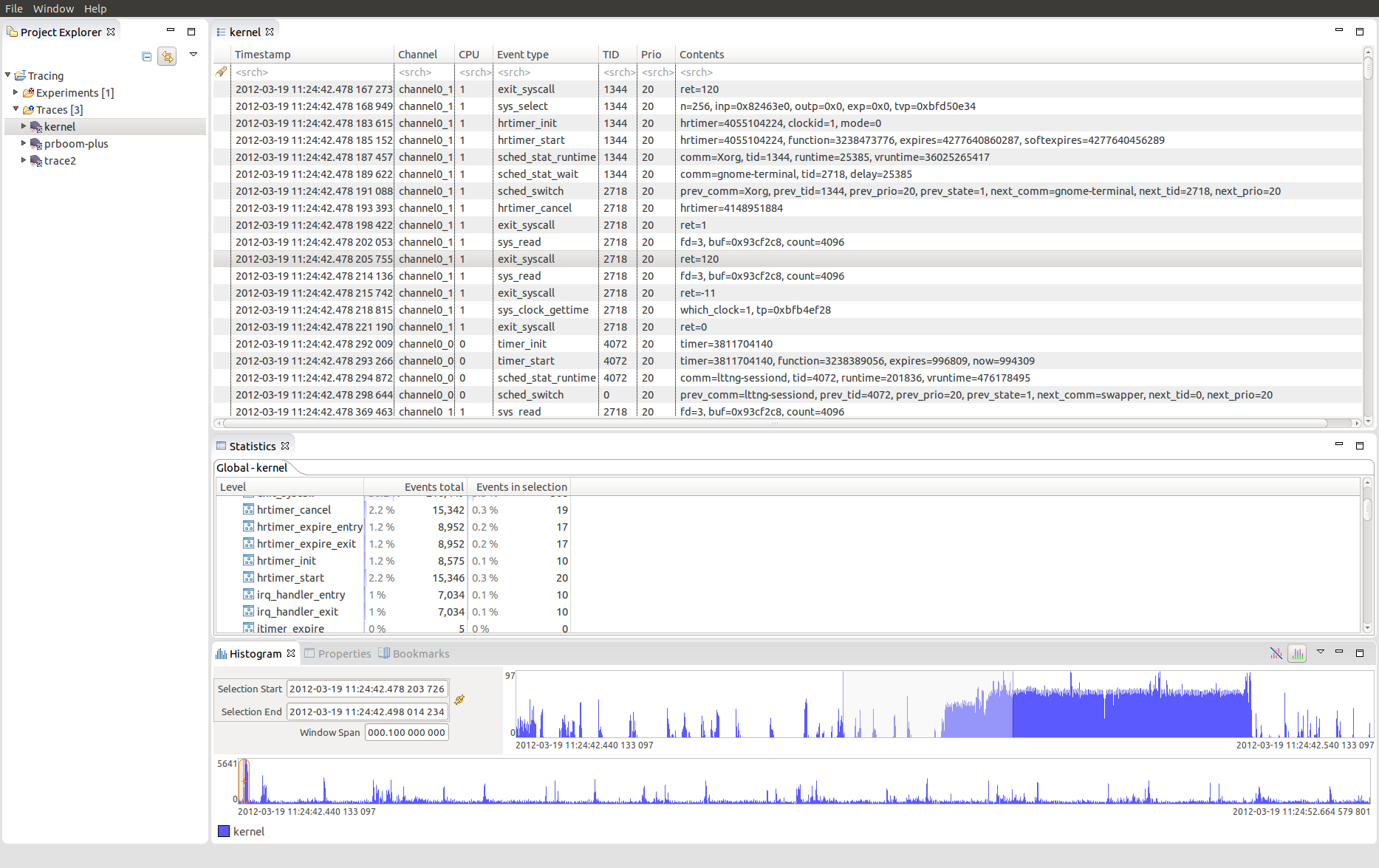
The Tracing perspective is part of the Tracing and Monitoring Framework (TMF) and groups the following views:
The views are synchronized i.e. selecting an event, a timestamp, a time range, etc will update the other views accordingly.
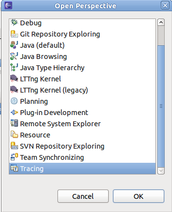
The perspective can be opened from the Eclipse Open Perspective dialog ( Window > Open Perspective... > Other).
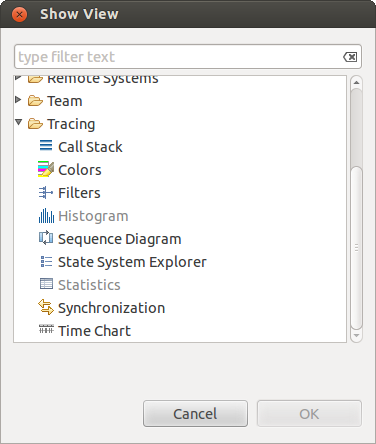
In addition to these views, the Tracing and Monitoring Framework (TMF) feature provides a set of generic tracing specific views, such as:
The framework also supports user creation of Custom Parsers.
To open one of the above Tracing views, use the Eclipse Show View dialog ( Window > Show View > Other...). Then select the relevant view from the Tracing category.
Additionally, the LTTng Control feature provides an LTTng Tracer Control functionality. It comes with a dedicated Control View.
The Project Explorer view is the standard Eclipse Project Explorer. Tracing projects are well integrated in the Eclipse's Common Navigator Framework. The Project Explorer shows Tracing project with a small "T" decorator in the upper right of the project folder icon.
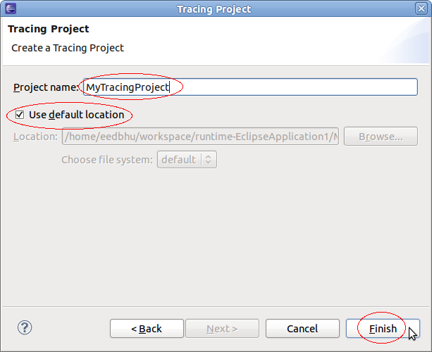
A new Tracing project can be created using the New Tracing Project wizard. To create a new Tracing select File > New > Project... from the main menu bar or alternatively form the context-sensitive menu (click with right mouse button in the Project Explorer.
The first page of project wizard will open.
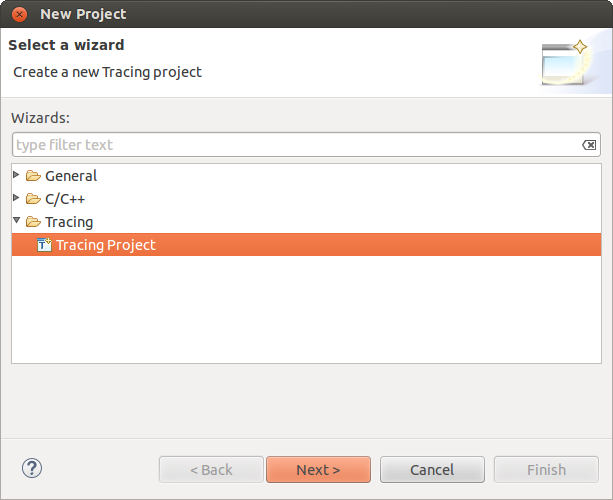
In the list of project categories, expand category Tracing and select Tracing Project and the click on Next >. A second page of the wizard will show. Now enter the a name in the field Project Name, select a location if required and the press on Finish.
A new project will appear in the Project Explorer view.
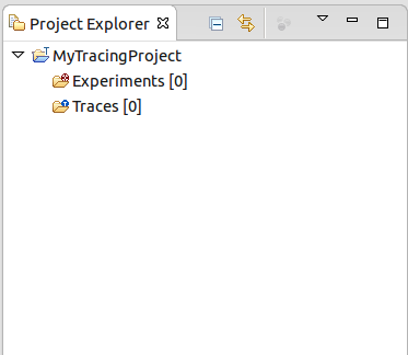
Tracing projects have two sub-folders: Traces which holds the individual traces, and Experiments which holds sets of traces that we want to correlate.
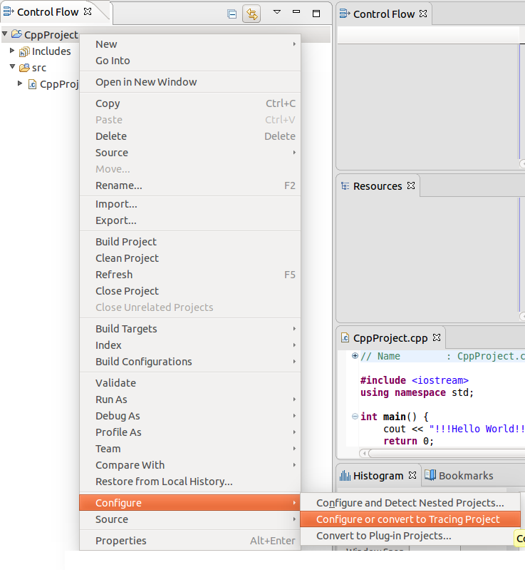
It is possible to configure an existing project, for example C/C++ or Java project, as a Tracing project. All Trace Compass related features will be available within the same project. To configure a project as Tracing project, right-click on the project in the Project Explorer and select menu item Configure > Configure or convert to Tracing Project.
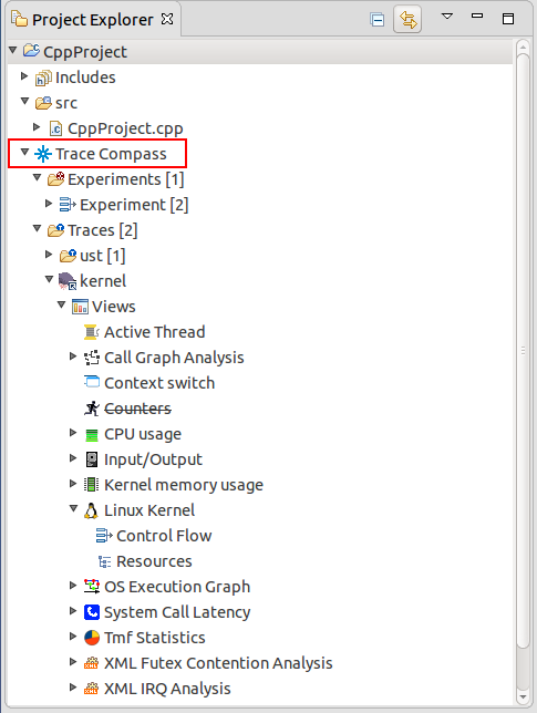
Upon successful configuration, the project tree will be updated and the Trace Compass top-level node will be added. Expanding the Trace Compass node will show the Traces and Experiments nodes from the Tracing project.
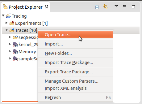
The Traces folder holds the set of traces available for a tracing project. It can optionally contain a tree of trace folders to organize traces into sub-folders. The following chapters will explain different ways to import traces to the Traces folder of a tracing project.
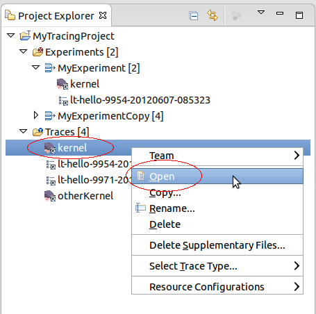
To open a trace, right-click on a target trace folder and select Open Trace....
A new dialog will show for selecting a trace to open. Select a trace file and then click on OK. Note that for traces that are directories (such as Common Trace Format (CTF) traces) any file in the trace directory can be selected to open the trace. Now, the trace viewer will attempt to detect the trace types of the selected trace. The auto detection algorithm will validate the trace against all known trace types. If multiple trace types are valid, a trace type is chosen based on a confidence criteria. The validation process and the computation of the confidence level are trace type specific. After successful validation the trace will be linked into the selected target trace folder and then opened with the detected trace type.
Depending of the trace types enabled in the Trace Types preference page, the list of available trace types can vary.
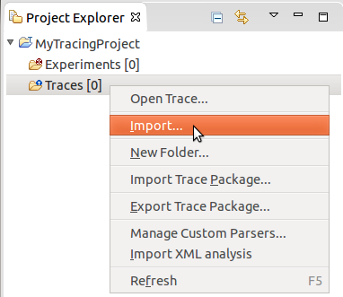
To import a set of traces to a trace folder, right-click on the target folder and select Import... from the context-sensitive menu.
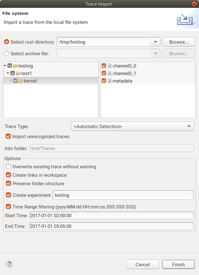
At this point, the Import Trace Wizard will show for selecting traces to import. By default, it shows the correct destination directory where the traces will be imported to. Now, specify the location of the traces in the Root directory. For that click on the button Browse, browse the media to the location of the traces and click on OK. Then select the traces to import in the list of files and folders. If the selected files include archive files (tar, zip), they will be extracted automatically and imported as well.
Traces can also be imported directly from an archive file such as a zip or a tar file by selecting the Select archive file option then by clicking Browse. Then select the traces to import in the list of files and folders as usual.
Optionally, select the Trace Type from the drop-down menu. If Trace Type is set to <Automatic Detection>, the wizard will attempt to detect the trace types of the selected files. The automatic detection algorithm validates a trace against all the trace types enabled in the Trace Types preference page. If multiple trace types are valid, a trace type is chosen based on a confidence criteria. The validation process and the computation of the confidence level are trace type specific. Optionally, Import unrecognized traces can be selected to import trace files that could not be automatically detected by <Automatic Detection>.
Select or deselect the checkboxes for Overwrite existing trace without warning, Create links in workspace and Preserve folder structure. When all options are configured, click on Finish.
Note that traces of certain types (e.g. LTTng Kernel) are actually a composite of multiple channel traces grouped under a folder. Either the folder or its files can be selected to import the trace.
The option Preserve folder structure will create, if necessary, the structure of folders relative to (and excluding) the selected Root directory (or Archive file) into the target trace folder.
The option Create Experiment will create an experiment with all imported traces. By default, the experiment name is the Root directory name, when importing from directory, or the Archive file name, when importing from archive. One can change the experiment name by typing a new name in the text box beside the option.
The option Time Range filtering will filter your previously selected traces using the given time range. A trace will be imported into the project only if its time range is included or overlap the provided range.
If a trace already exists with the same name in the target trace folder, the user can choose to rename the imported trace, overwrite the original trace or skip the trace. When rename is chosen, a number is appended to the trace name, for example smalltrace becomes smalltrace(2).
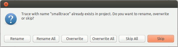
If one selects Rename All, Overwrite All or Skip All the choice will be applied for all traces with a name conflict.
Upon successful importing, the traces will be stored in the target trace folder. If a trace type was associated to a trace, then the corresponding icon will be displayed. If no trace type is detected the default editor icon associated with this file type will be displayed. Linked traces will have a little arrow as decorator on the right bottom corner.
Depending of the trace types enabled in the Trace Types preference page, the list of available trace types can vary.
Alternatively, one can open the Import... menu from the File main menu, then select Tracing > Trace Import and click on Next >.
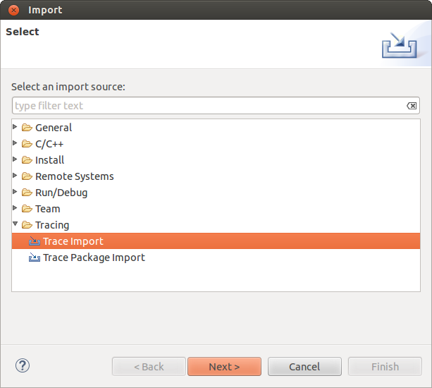
At this point, the Import Trace Wizard will show. To import traces to the tracing project, follow the instructions that were described above.
Traces can be also be imported to a project by dragging from another tracing project and dropping to the project's target trace folder. The trace will be copied and the trace type will be set.
Any resource can be dragged and dropped from a non-tracing project, and any file or folder can be dragged from an external tool, into a tracing project's trace folder. The resource will be copied or imported as a new trace and it will be attempted to detect the trace types of the imported resource. The automatic detection algorithm validates a trace against all known trace types. If multiple trace types are valid, a trace type is chosen based on a confidence criteria. The validation process and the computation of the confidence level are trace type specific. If no trace type is detected the user needs to set the trace type manually.
To import the trace as a link, use the platform-specific key modifier while dragging the source trace. A link will be created in the target project to the trace's location on the file system.
If a folder containing traces is dropped on a trace folder, the full directory structure will be copied or linked to the target trace folder. The trace type of the contained traces will not be auto-detected.
It is also possible to drop a trace, resource, file or folder into an existing experiment. If the item does not already exist as a trace in the project's trace folder, it will first be copied or imported, then the trace will be added to the experiment.
A trace package is an archive file that contains the trace itself and can also contain its bookmarks and its supplementary files. Including supplementary files in the package can improve performance of opening an imported trace but at the expense of package size.
The Export Trace Package Wizard allows users to select a trace and export its files and bookmarks to an archive on a media.
The Traces folder holds the set of traces available for a tracing project. To export traces contained in the Traces folder, one can open the Export... menu from the File main menu. Then select Trace Package Export
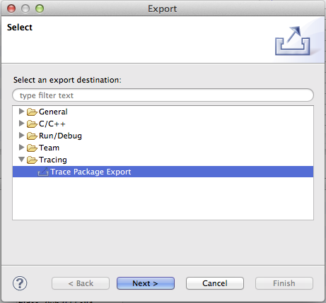
At this point, the Trace Package Export is opened. The project containing the traces has to be selected first then the traces to be exported.
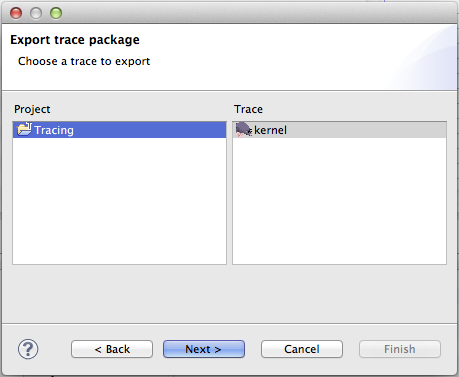
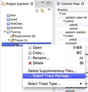
One can also open the wizard and skip the first page by expanding the project, selecting traces or trace folders under the Traces folder, then right-clicking and selecting the Export Trace Package... menu item in the context-sensitive menu.
Next, the user can choose the content to export and various format options for the resulting file.
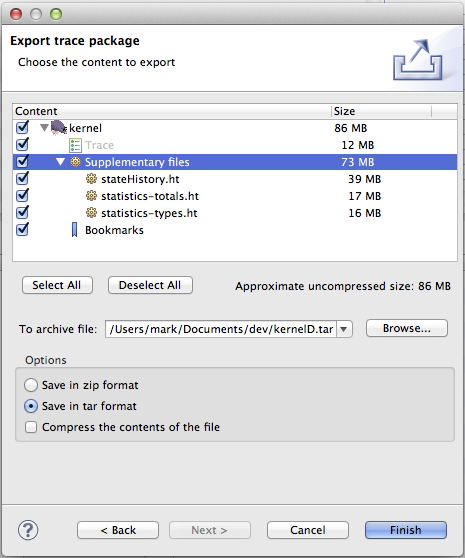
The Trace item is always selected and represents the files that constitute the trace. The Supplementary files items represent files that are typically generated when a trace is opened by the viewer. Sharing these files can speed up opening a trace dramatically but also increases the size of the exported archive file. The Size column can help to decide whether or not to include these files. Lastly, by selecting Bookmarks, the user can export all the bookmarks so that they can be shared along with the trace.
The To archive file field is used to specify the location where to save the resulting archive.
The Options section allows the user to choose between a tar archive or a zip archive. Compression can also be toggled on or off.
When Finish button is clicked, the package is generated and saved to the media. The folder structure of the selected traces relative to the Traces folder is preserved in the trace package.
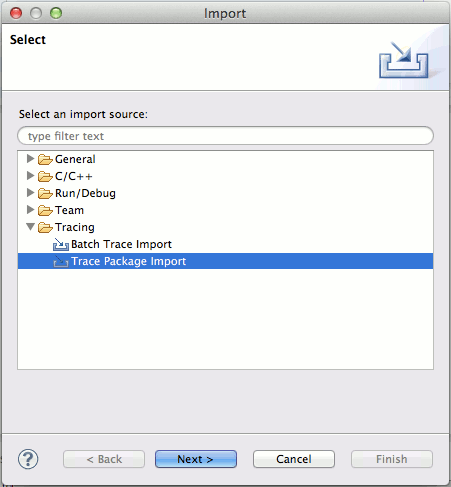
The Import Trace Package Wizard allows users to select a previously exported trace package from their media and import the content of the package in the workspace.
The Traces folder holds the set of traces for a tracing project. To import a trace package to the Traces folder, one can open the Import... menu from the File main menu. Then select Trace Package Import.
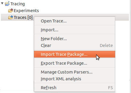
One can also open the wizard by expanding the project name, right-clicking on a target folder under the Traces folder then selecting Import Trace Package... menu item in the context-sensitive menu.
At this point, the Trace Package Import Wizard is opened.
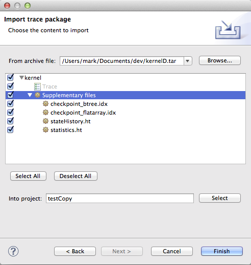
The From archive file field is used to specify the location of the trace package to export. The user can choose the content to import in the tree.
If the wizard was opened using the File menu, the destination project has to be selected in the Into project field.
When Finish is clicked, the trace is imported in the target folder. The folder structure from the trace package is restored in the target folder.
Traces and trace folders in the workspace might be updated on the media. To refresh the content, right-click the trace or trace folder and select menu item Refresh. Alternatively, select the trace or trace folder and press key F5.
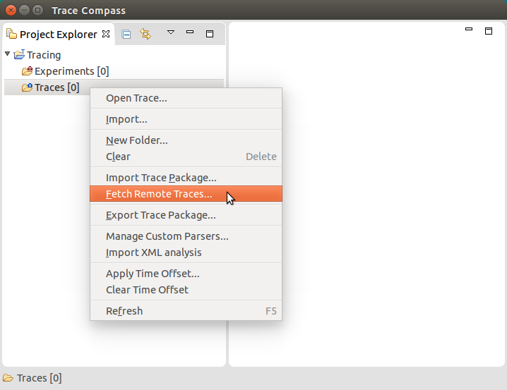
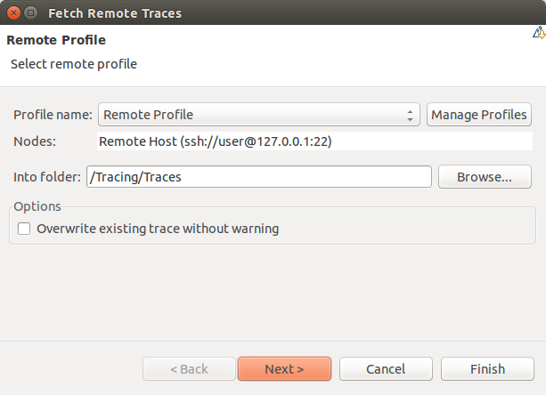
It is possible to import traces automatically from one or more remote hosts according to a predefined remote profile by using the Fetch Remote Traces wizard.
To start the wizard, right-click on a target trace folder and select Fetch Remote Traces....
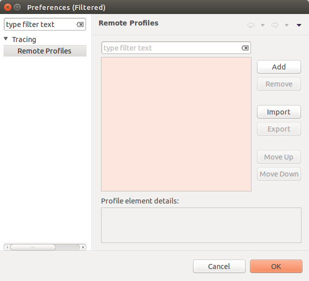
The wizard opens on the Remote Profile page.
![]()
If the remote profile already exists, it can be selected in the Profile name combo box. Otherwise, click Manage Profiles to open the Remote Profiles preferences page.
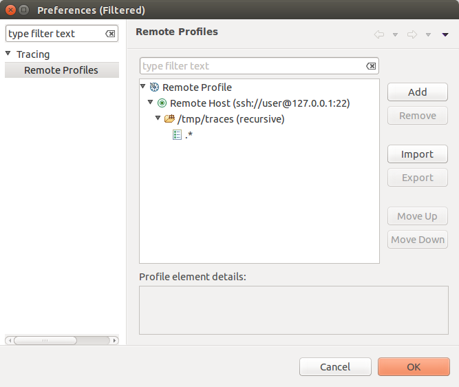
Click Add to create a new remote profile. A default remote profile template appears.
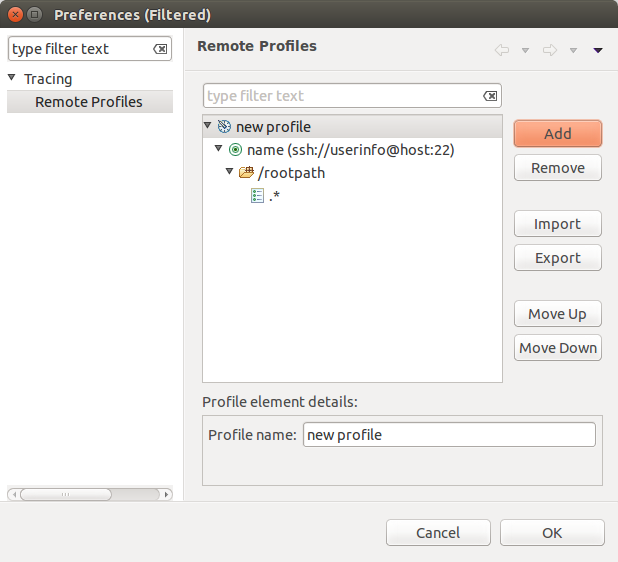
Edit the Profile name field to give a unique name to the new profile.
Under the Profile element, at least one Connection Node element must be defined.
Node name: Unique name for the connection within the scope of the Remote Services provider.
URI: URI for the connection. Its scheme maps to a particular Remote Services provider. If the connection name already exists for that provider, the URI must match its connection information. The scheme ssh can be used for the Built-In SSH provider. The scheme file can be used for the local file system.
To view or edit existing connections, see the Remote Development > Remote Connections preferences page. On this page the user can enter a password for the connection.
Under the Connection Node element, at least one Trace Group element must be defined.
Root path: The absolute root path from where traces will be fetched. For example, /home/user or /C/Users/user.
Recursive: Check this box to search for traces recursively in the root path.
Under the Trace Group element, at least one Trace element must be defined.
File pattern: A regular expression pattern to match against the file name of traces found under the root path. If the Recursive option is used, the pattern must match against the relative path of the trace, using forward-slash as a path separator. Files that do not match this pattern are ignored. If multiple Trace elements have a matching pattern, the first matching element will be used, and therefore the most specific patterns should be listed first. Following are some pattern examples:
.*matches any trace in any folder
[^/]*\.logmatches traces with .log extension in the root path folder
.*\.logmatches traces with .log extension in any folder
folder-[^/]*/[^/]*\.logmatches traces with .log extension in folders matching a pattern
(.*/)?filenamematches traces with a specific name in any folder
Trace Type: The trace type to assign to the traces after fetching, or <Automatic Detection> to determine the trace type automatically. Note that traces whose trace type can not be assigned according to this setting are not deleted after fetching.
Right-click a profile element to bring up its context menu. A New child element of the appropriate type can be created. Select Delete to delete a node, or Cut, Copy and Paste to move or copy elements from one profile element to another. The keyboard shortcuts can also be used.
Press the Add button to create a new element of the same type and following the selected element, or a new profile if the selection is empty.
Press the Remove button to delete the selected profile elements.
Press the Import button to import profiles from a previously exported XML file.
Press the Export button to export the selected profiles to an XML file.
Press the Move Up or Move Down buttons to reorder the selected profile element.
The filter text box can be used to filter profiles based on the profile name or connection node.
When the remote profile information is valid and complete, press the OK button to save the remote profiles preferences.
Back in the Remote Profiles wizard page, select the desired profile and click Next >. Clicking Finish at this point will automatically select and download all matching traces.
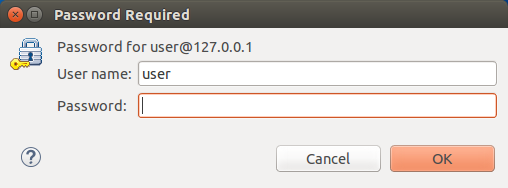
If required, the selected remote connections are created and connection is established. The user may be prompted for a password. This can be avoided by storing the password for the connection in the Remote Connections preference page.
The root path of every Trace Group is scanned for matching files. The result is shown in the Remote Traces wizard page.
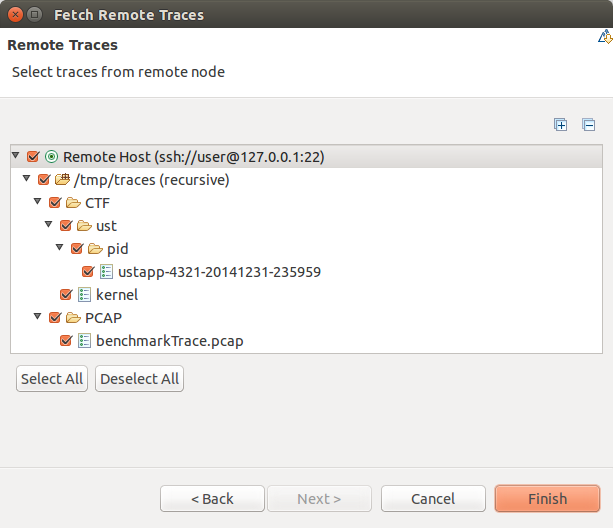
Select the traces to fetch by checking or unchecking the desired connection node, trace group, folder or individual trace. Click Finish to complete the operation.
If any name conflict occurs, the user will be prompted to rename, overwrite or skip the trace, unless the Overwrite existing trace without warning option was checked in the Remote Profiles wizard page.
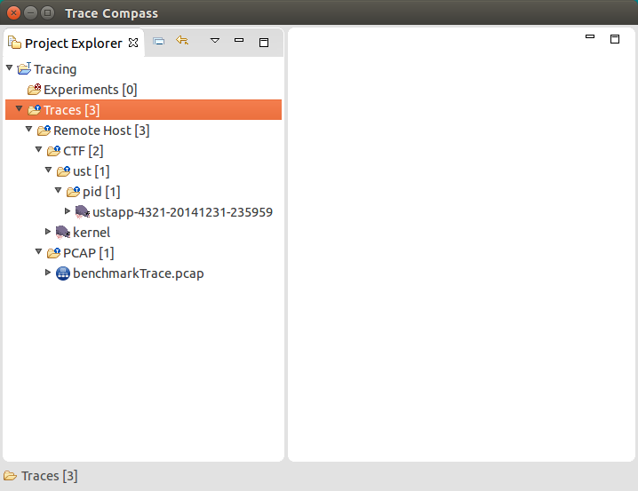
The downloaded traces will be imported to the initially selected project folder. They will be stored under a folder structure with the pattern <connection name>/<path>/<trace name> where the path is the trace's remote path relative to its trace group's root path.
If no trace type was selected a trace type has to be associated to a trace before it can be opened. To select a trace type select the relevant trace and click the right mouse button. In the context-sensitive menu, select Select Trace Type... menu item. A sub-menu will show will all available trace type categories. From the relevant category select the required trace type. The examples, below show how to select the Common Trace Format types Linux Kernel Trace and Generic CTF trace.
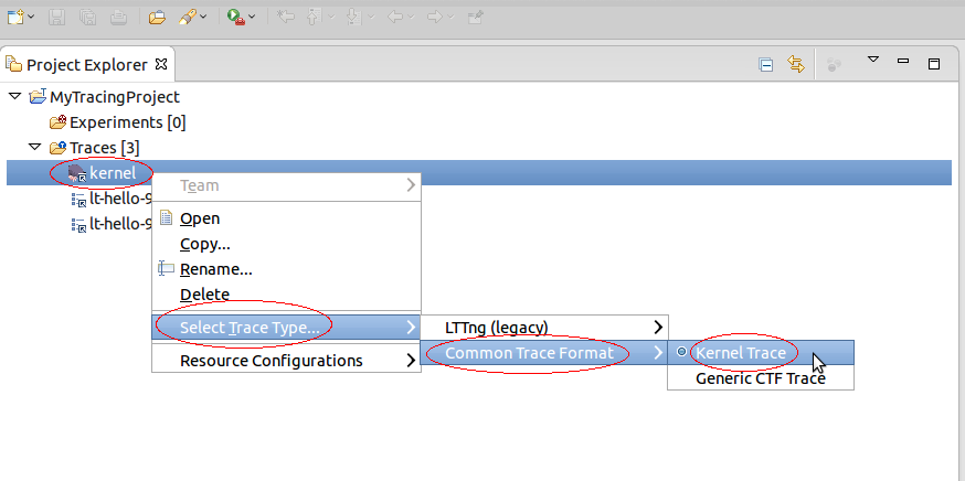
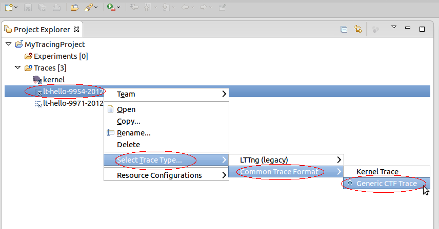
After selecting the trace type, the trace icon will be updated with the corresponding trace type icon.
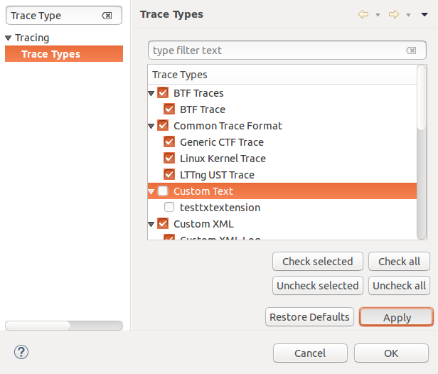
The user can edit the Trace Types preference page to choose which trace types will be available under the Select Trace Type... menu.
The Trace Types preference page lists all the available trace types and allows the user to enable/disable the trace types.
Trace type is an extension point of the Tracing and Monitoring Framework (TMF). Depending on which features are loaded and which custom parsers have been created, the list of trace types can vary.
The user needs to press the Apply button or OK' to save the changes.
Only the enabled trace types will be used for trace importing, auto-detection, as well as shown under the Select Trace Type... menu.
To access the Trace Types preference page, select the Window menu. Then Select Preferences and search for Trace Type under Tracing group. The example below shows the Trace Types preference page.
A trace or experiment can be opened by double-clicking the left mouse button on the trace or experiment in the Project Explorer view. Alternatively, select the trace or experiment in the in the Project Explorer view and click the right mouse button. Then select Open menu item of the context-sensitive menu. If there is no trace type set for a file resource then the file will be opened in the default editor associated with this file type.
If there is a default perspective associated with the opened trace or experiment and it is not the active perspective, the user will be prompted to switch to this perspective. The user can choose to remember this decision. The user preference can be later updated in the Perspectives preference page. Select Window > Preferences in the main menu, then select Tracing > Perspectives in the tree, and choose one of the options under Open the associated perspective when a trace is opened..
When opening a trace or experiment, all currently opened views which are relevant for the corresponding trace type will be updated.
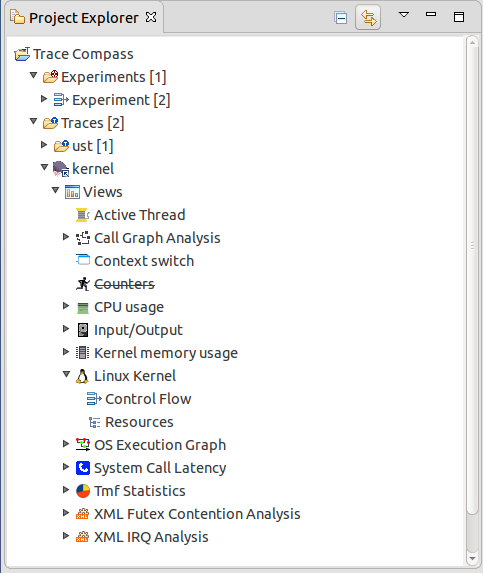
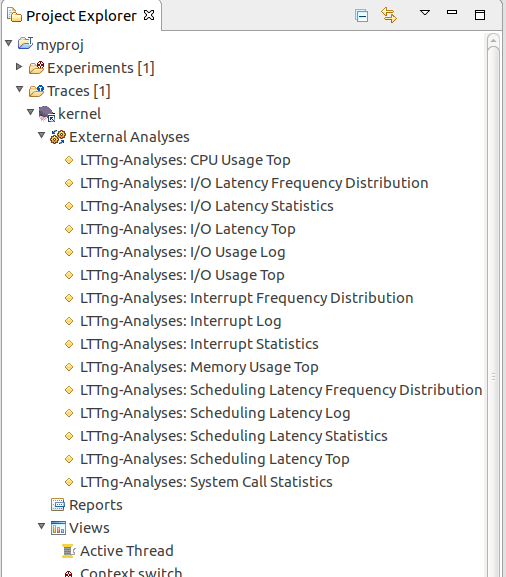
The Project Explorer tree for the opened trace will be updated and will show all the available analysis for and views for the corresponding trace type as in the following image.
If an analysis can't be executed (e.g. due to missing required events) then the analysis will be strike-through. Right-mouse clicking on the analysis tree element and selecting menu item Help, will provide more details why the analysis can't be executed.
Double-clicking the left mouse button on the a analysis, will execute the analysis. Alternatively, select an analysis in the in the Project Explorer view and click the right mouse button. Then select Open menu item of the context-sensitive menu. Opening a view tree element underneath the analysis will also trigger the execution of the corresponding analysis.
Note, that some analysis are implemented for automatic execution, so that they are executed when opening the trace.
If a trace resource is a file (and not a directory), then the Open With menu item is available in the context-sensitive menu and can be used to open the trace source file with any applicable internal or external editor. In that case the trace will not be processed by the tracing application.
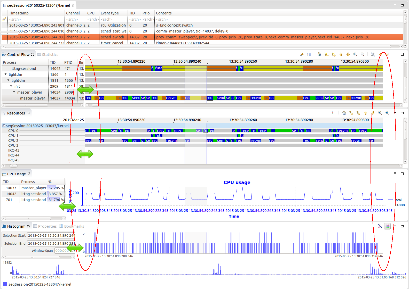
An experiment consists in an arbitrary number of aggregated traces for purpose of correlation. In the degenerate case, an experiment can consist of a single trace. The experiment provides a unified, time-ordered stream of the individual trace events.
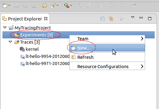
To create an experiment, select the folder Experiments and click the right mouse button. Then select New....
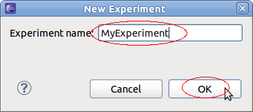
A new display will open for entering the experiment name. Type the name of the experiment in the text field Experiment Name and the click on OK.
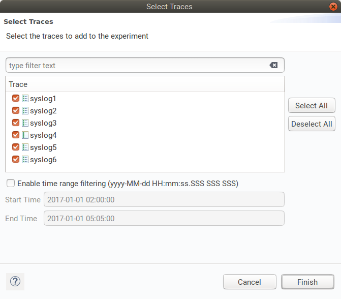
After creating an experiment, traces need to be added to the experiment. To select traces for an experiment select the newly create experiment and click the right mouse button. Select Select Traces... from the context sensitive menu.
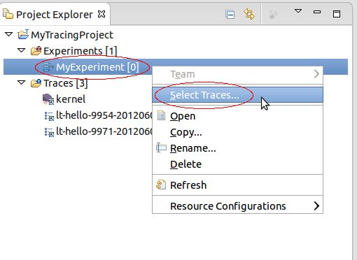
A new dialog box will open with a list of available traces. The filter text box can be used to quickly find traces. Use buttons Select All or Deselect All to select or deselect all traces. Select the traces to add from the list and then click on Finish or you can go a step further by activating the time range filtering option. Enter the time range using the following format: 'yyyy-MM-dd HH:mm:ss.SSS SSS SSS' and click on Finish. By using this option, only traces, among your selected trace, that are in or overlap the range will be added to the experiment.
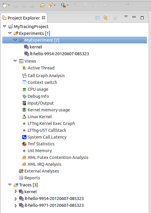
Now the selected traces will be linked to the experiment and will be shown under the Experiments folder. Expanding of the Views folder will show all available analysis that are defined either for the experiment or for contained traces. If there are multiple traces of the same trace type the "Views" folder will aggregate all available analysis that are the same to one entry in the tree. Each analysis output (view) can be opened from the experiment context.
Alternatively, traces can be added to an experiment using Drag and Drop.
An experiment can be quickly created and opened automatically by selecting one or more traces and/or trace folders in the Project Explorer view, and then selecting the Open as Experiment... context menu. A sub-menu with the available experiment types is opened. Select the desired experiment type from the sub-menu. All selected traces and traces recursively found in selected trace folders will be added to the experiment.
If a single trace or trace folder is selected, its name will be used for the experiment, otherwise a default name will be used, possibly appended with a number to avoid name clashes.
If an experiment with the same name and traces already exists, it will be reopened (or selected if it is already opened). Otherwise, a new experiment will be created and opened.
To remove one or more traces from an experiment select the trace(s) to remove under the Experiment folder and click the right mouse button. Select Remove from the context sensitive menu.
After that the selected trace(s) are removed from the experiment. Note that the traces are still in the Traces folder.
To delete one or more traces from an experiment select the trace(s) to delete under the Experiment folder and click the right mouse button. Select Delete from the context sensitive menu.
After that, the selected trace(s) are removed from the experiment. Note that the traces are also deleted from the Traces folder.
Traces and Experiment can be renamed from the Project Explorer view. To rename a trace or experiment select the relevant trace and click the right mouse button. Then select Rename... from the context sensitive menu. The trace or experiment needs to be closed in order to do this operation.
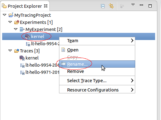
A new dialog box will show for entering a new name. Enter a new trace or experiment name respectively in the relevant text field and click on OK. If the new name already exists the dialog box will show an error and a different name has to be entered.
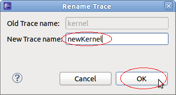
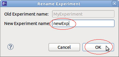
After successful renaming the new name will show in the Project Explorer. In case of a trace all reference links to that trace will be updated too. Note that linked traces only changes the display name, the underlying trace resource will stay the original name.
Note that all supplementary files will be also handled accordingly (see also Deleting Supplementary Files).
To copy a trace or experiment select the relevant trace or experiment in the Project Explorer view and click the right mouse button. Then select Copy... from the context sensitive menu.
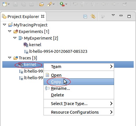
A new dialog box will show for entering a new name. Enter a new trace or experiment name respectively in the relevant text field and click on OK. In case of a linked trace two options are available, Copy as a link or Copy as a new trace. The first option, default one, the copied trace will be a link to the original trace. The second option, will make a copy of the original trace in your workspace. If the new name already exists the dialog box will show an error and a different name has to be entered.
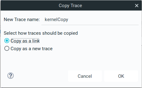
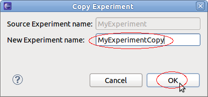
After successful copy operation the new trace or experiment respectively will show in the Project Explorer.
Note that the directory for all supplementary files will be copied, too. (see also Deleting Supplementary Files).
To delete a trace or experiment select the relevant trace or experiment in the Project Explorer view and click the right mouse button. Then select Delete... from the context sensitive menu. The trace or experiment needs to be closed in order to do this operation.
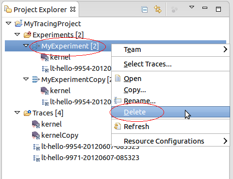
A confirmation dialog box will open. To perform the deletion press OK otherwise select Cancel.
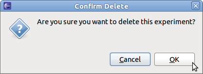
After successful operation the selected trace or experiment will be removed from the project. In case of a linked trace only the link will be removed. The actual trace resource remain on the disk.
Note that the directory for all supplementary files will be deleted, too. (see also Deleting Supplementary Files).
Supplementary files are by definition trace specific files that accompany a trace. These file could be temporary files, persistent indexes or any other persistent data files created by the LTTng integration in Eclipse during parsing a trace. For the LTTng 2.0 trace viewer a persistent state history of the Linux Kernel is created and is stored under the name stateHistory.ht. The statistics for all traces are stored under statistics.ht. Other state systems may appear in the same folder as more custom views are added.
All supplementary file are hidden from the user and are handled internally by the TMF. However, there is a possibility to delete the supplementary files so that they are recreated when opening a trace.
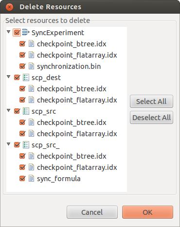
To delete all supplementary files from one or many traces and experiments, select the relevant traces and experiments in the Project Explorer view and click the right mouse button. Then select the Delete Supplementary Files... menu item from the context-sensitive menu.
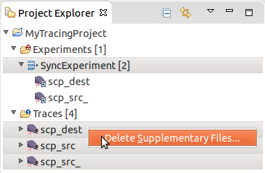
A new dialog box will open with a list of supplementary files, grouped under the trace or experiment they belong to. Select the file(s) to delete from the list and press OK. The traces and experiments that need to be closed in order to do this operation will automatically be closed.
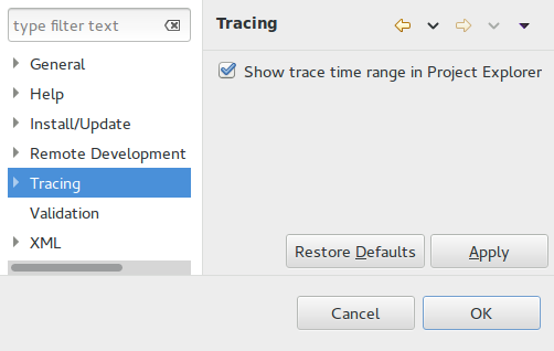
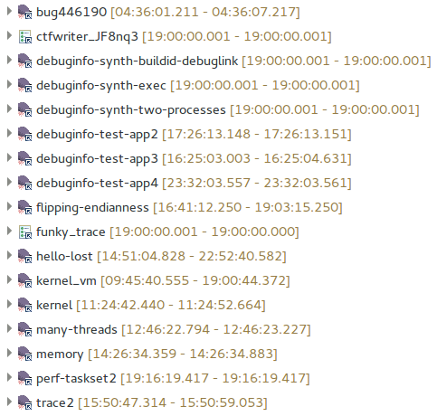
The trace's time range can be displayed alongside the trace's name. The time is displayed in the Time Format from Tracing preferences.
To enable this feature, head to Preferences > Tracing and check the box Show trace time range in Project Explorer.
If a trace is empty or its type unknown, nothing will be shown. It the range has not been fully read from the trace or the supplementary files, [...] will be shown. If the trace is being read and only its start time start is known, [start - ...] will be shown. Finally, when the end time end is also known, [start - end] will be shown.
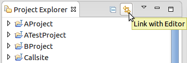
The tracing projects support the feature
Link With Editor of the Project Explorer view. With this feature it is now possible to
To enable or disable this feature toggle the Link With Editor button of the Project Explorer view as shown below.
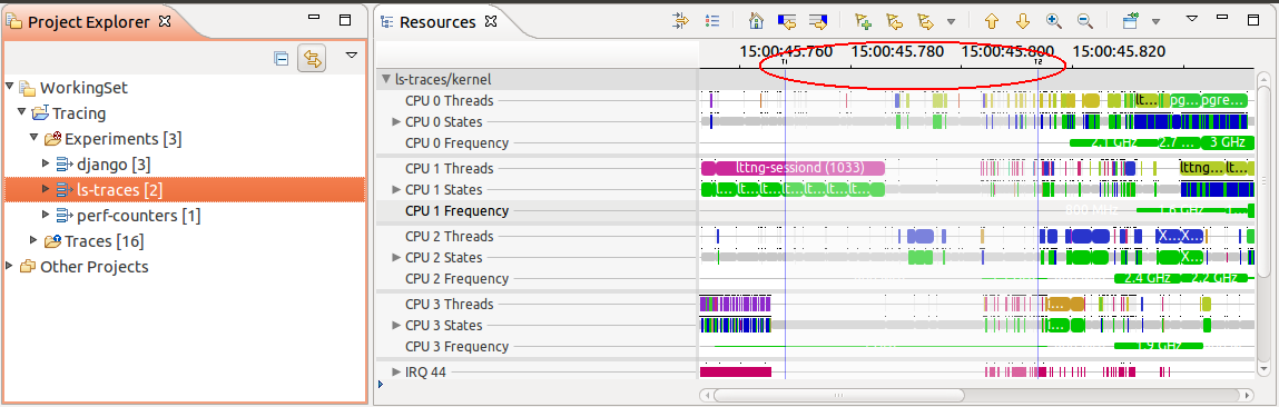
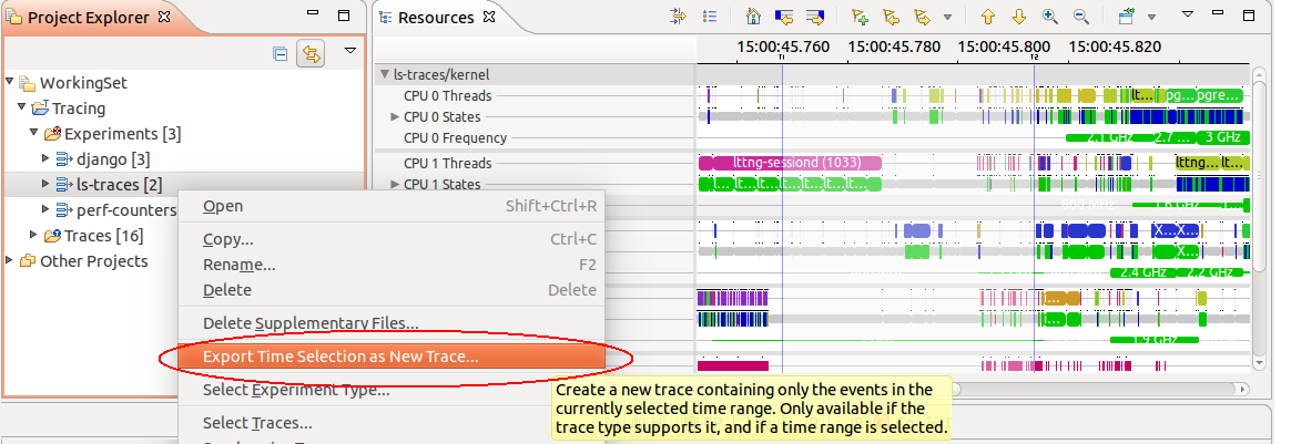
If a time range (not a single timestamp) is selected in any of the time-based views, right clicking on the trace or experiment element in the Project Explorer will show Export Time Selection as New Trace. This option allows trimming the current trace to a subset of its events, while preserving all the states that may have been computed by various analyses using events present before the exported time range.
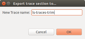
The Exporting Time Selection as New Trace option will create a new trace and import it into the current tracing project. A selection dialog will be presented to the user to define where the new trace should be written. This is where the new trace files will be written, as well as any appropriate initial state files.
The new trace will be initially named the same as the original. The user must then free to rename the new trace. The trace can also be removed from the project and re-imported later with no loss of information.
Note: Since trace writing works differently for every trace type, the trimming feature has to be implemented for the target trace's type. If the option remains grayed out even if a time range is selected, it is because the given trace type does not implement the trim feature.
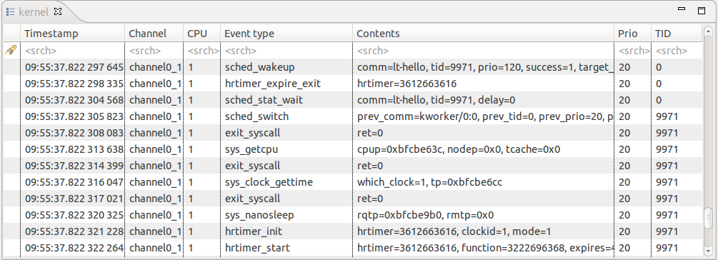
The Events editor shows the basic trace data elements (events) in a tabular format. The editors can be dragged in the editor area so that several traces may be shown side by side. These traces are synchronized by timestamp.
The header displays the current trace (or experiment) name.
The columns of the table are defined by the fields (aspects) of the specific trace type. These are the defaults:
The first row of the table is the header row a.k.a. the Search and Filter row.
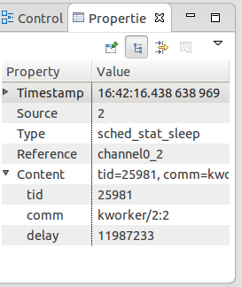
The highlighted event is the current event and is synchronized with the other views. If you select another event, the other views will be updated accordingly. The properties view will display a more detailed view of the selected event.
An event range can be selected by holding the Shift key while clicking another event or using any of the cursor keys ( Up', Down, PageUp, PageDown, Home, End). The first and last events in the selection will be used to determine the current selected time range for synchronization with the other views.
The Events editor can be closed, disposing a trace. When this is done, all the views displaying the information will be updated with the trace data of the next event editor tab. If all the editor tabs are closed, then the views will display their empty states.
Column order and size is preserved when changed. If a column is lost due to it being resized to 0 pixels, right click on the context menu and select Show All, it will be restored to a visible size.
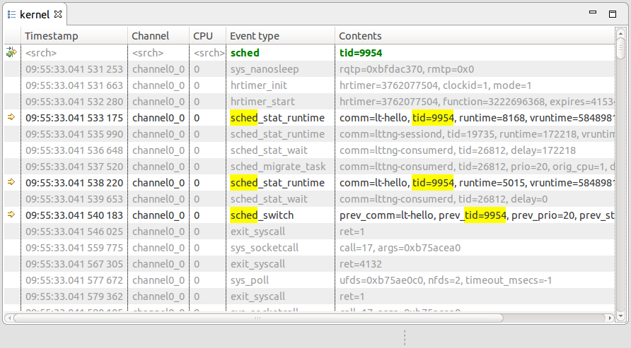
Searching and filtering of events in the table can be performed by entering matching conditions in one or multiple columns in the header row (the first row below the column header).
To apply a matching condition to a specific column, click on the column's header row cell, type in a regular expression. You can also enter a simple text string and it will be automatically be replaced with a 'contains' regular expression.
Press the Enter key to apply the condition as a search condition. It will be added to any existing search conditions.
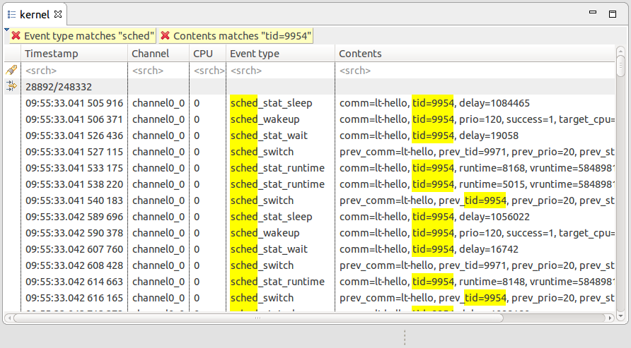
Press the Ctrl+Enter key to immediately add the condition (and any other existing search conditions) as a filter instead.
When matching conditions are applied to two or more columns, all conditions must be met for the event to match (i.e. 'and' behavior).
A preset filter created in the Filters view can also be applied by right-clicking on the table and selecting Apply preset filter... > filter name
When a searching condition is applied to the header row, the table will select the next matching event starting from the top currently displayed event. Wrapping will occur if there is no match until the end of the trace.
All matching events will have a 'search match' icon in their left margin. Non-matching events will be dimmed. The characters in each column which match the regular expression will be highlighted.
Pressing the Enter key will search and select the next matching event. Pressing the Shift+Enter key will search and select the previous matching event. Wrapping will occur in both directions.
Press Esc to cancel an ongoing search.
To add the currently applied search condition(s) as filter(s), click the
Add as Filter
 button in the header row margin, or press the
Ctrl+Enter key.
button in the header row margin, or press the
Ctrl+Enter key.
Press Delete to clear the header row and reset all events to normal.
When a new filter is applied, the table will clear all events and fill itself with matching events as they are found from the beginning of the trace. The characters in each column which match the regular expression will be highlighted.
A status row will be displayed before and after the matching events, dynamically showing how many matching events were found and how many events were processed so far. Once the filtering is completed, the status row icon in the left margin will change from a 'stop' to a 'filter' icon.
Press Esc to stop an ongoing filtering. In this case the status row icon will remain as a 'stop' icon to indicate that not all events were processed.
The header bar will be displayed above the table and will show a label for each applied filter. Clicking on a label will highlight the matching strings in the events that correspond to this filter condition. Pressing the Delete key will clear this highlighting.
To remove a specific filter, click on the
 icon on its label in the header bar. The table will be updated with the events matching the remaining filters.
The header bar can be collapsed and expanded by clicking on the

 icons in the top-left corner or on its background. In collapsed mode, a minimized version of the filter labels will be shown that can also be used to highlight or remove the corresponding filter.
Right-click on the table and select Clear Filters from the context menu to remove all filters. All trace events will be now shown in the table. Note that the currently selected event will remain selected even after the filters are removed.
You can also search on the subset of filtered events by entering a search condition in the header row while a filter is applied. Searching and filtering conditions are independent of each other.
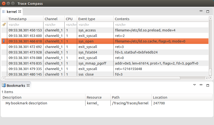
Any event of interest can be tagged with a bookmark.
To add a bookmark, double-click the left margin next to an event, or right-click the margin and select Add bookmark.... Alternatively use the Edit > Add bookmark... menu. Edit the bookmark description as desired and press OK.
The bookmark will be displayed in the left margin, and hovering the mouse over the bookmark icon will display the description in a tooltip.
The bookmark will be added to the Bookmarks view. In this view the bookmark description can be edited, and the bookmark can be deleted. Double-clicking the bookmark or selecting Go to from its context menu will open the trace or experiment and go directly to the event that was bookmarked.
To remove a bookmark, double-click its icon, select Remove Bookmark from the left margin context menu, or select Delete from the Bookmarks view.
The text of selected events can be copied to the clipboard by right-clicking on the table and selecting Copy to Clipboard in the context menu. The clipboard contents will be prefixed by the column header names. For every event in the table selection, the column text will be copied to the clipboard. The column text will be tab-separated. Hidden columns will not be included in the clipboard contents.
Some trace types can optionally embed information in the trace to indicate the source of a trace event. This is accessed through the event context menu by right-clicking on an event in the table.
If a source file is available in the trace for the selected event, the item Open Source Code is shown in the context menu. Selecting this menu item will attempt to find the source file in all opened projects in the workspace. If multiple candidates exist, a selection dialog will be shown to the user. The selected source file will be opened, at the correct line, in its default language editor. If no candidate is found, an error dialog is shown displaying the source code information.
If an EMF model URI is available in the trace for the selected event, the item Open Model Element is shown in the context menu. Selecting this menu item will attempt to open the model file in the project specified in the URI. The model file will be opened in its default model editor. If the model file is not found, an error dialog is shown displaying the URI information.
It is possible to export the content of the trace to a text file based on the columns displayed in the events table. If a filter (see Filtering ) was defined prior exporting only events that match the filter will be exported to the file. To export the trace to text, press the right mouse button on the events table. A context-sensitive menu will show. Select the Export To Text... menu option. A file locater dialog will open. Fill in the file name and location and then press on OK. A window with a progress bar will open till the export is finished.
Note: The columns in the text file are separated by tabs.
It's possible to refresh the content of the trace and resume indexing in case the current open trace was updated on the media. To refresh the trace, right-click into the table and select menu item Refresh. Alternatively, press key F5.
The implementation for collapsing of repetitive events is trace type specific and is only available for certain trace types. For example, a trace type could allow collapsing of consecutive events that have the same event content but not the same timestamp. If a trace type supports this feature then it is possible to select the Collapse Events menu item after pressing the right mouse button in the table.
When the collapsing of events is executing, the table will clear all events and fill itself with all relevant events. If the collapse condition is met, the first column of the table will show the number of times this event was repeated consecutively.
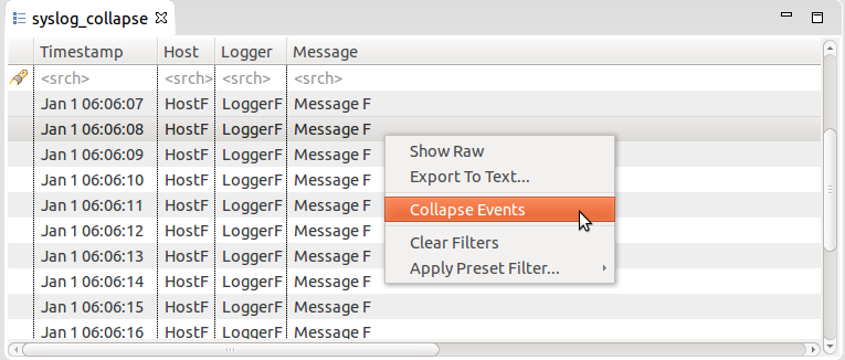
A status row will be displayed before and after the events, dynamically showing how many non-collapsed events were found and how many events were processed so far. Once the collapsing is completed, the status row icon in the left margin will change from a 'stop' to a 'filter' icon.
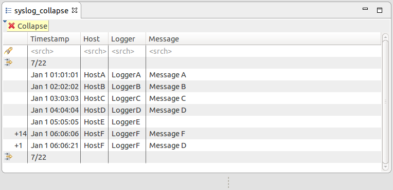
To remove the collapse filter, press the (
) icon on the
Collapse label in the header bar, or press the right mouse button in the table and select menu item
Clear Filters in the context sensitive menu (this will also remove any other filters).
The table columns can be reordered by the user by dragging the column headers. This column order is saved when the editor is closed. The setting applies to all traces of the same trace type.
The table columns can be hidden or restored by right-clicking on any column header and clicking on an item in the context menu to toggle its state. Clicking Show All will restore all table columns.
The table font can be customized by the user by changing the preference in Window > Preferences > General > Appearance > Colors and Fonts > Tracing > Trace event table font.
The search and filter highlight color can be customized by the user by changing the preference in Window > Preferences > General > Appearance > Colors and Fonts > Tracing > Trace event table highlight color.
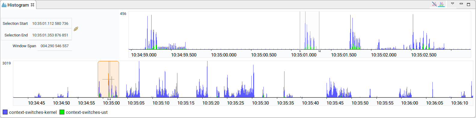
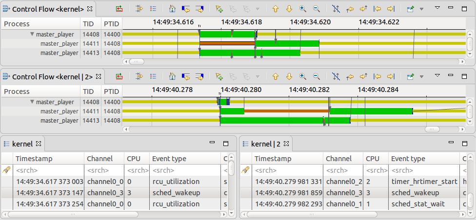
The Histogram View displays the trace events distribution with respect to time. When streaming a trace, this view is dynamically updated as the events are received. The time axis is aligned with other views that support automatic time axis alignment (see Automatic Time Axis Alignment).
The
Align Views toggle button
 in the view menu allows to disable and enable the automatic time axis alignment of time-based views. Disabling the alignment in the Histogram view will disable this feature across all the views because it's a workspace preference.
The
Hide Lost Events toggle button
 in the local toolbar allows to hide the bars of lost events. When the button is selected it can be toggled again to show the lost events.
The
Activate Trace Coloring toggle button
 in the local toolbar allows to use separate colors for each trace of an experiment. Note that this feature is not available if your experiment contains more than twenty two traces. When activated, a legend is displayed at the bottom on the histogram view.
On the top left, there are three text controls:
The controls can be used to modify their respective value. After validation, the other controls and views will be synchronized and updated accordingly. To modify both selection times simultaneously, press the link icon
which disables the
Selection End control input.
The large (full) histogram, at the bottom, shows the event distribution over the whole trace or set of traces. It also has a smaller semi-transparent orange window, with a cross-hair, that shows the current zoom window.
The smaller (zoom) histogram, on top right, corresponds to the current zoom window, a sub-range of the event set. The window size can be adjusted by dragging the sash left beside the zoom window.
The x-axis of each histogram corresponds to the event timestamps. The axis is now the same as the other views for a better visualization of the range. The y-axis shows the maximum number of events in the corresponding histogram bars.
The vertical blue line(s) show the current selection time (or range). If applicable, the region in the selection range will be shaded. In addition, when a selection is performed the status line (line placed at the very left bottom corner of Trace Compass) is now updated with the cursor position, the selection time or range and the delta for a range.

The mouse can be used to control the histogram:
Hovering the mouse over an histogram bar pops up an information window that displays the start/end time of the corresponding bar, as well as the number of events (and lost events) it represents. If the mouse is over the selection range, the selection span in seconds is displayed.
In each histogram, the following keys are handled:
The Statistics View displays the various event counters that are collected when analyzing a trace. After opening a trace, the element Statistics is added under the Tmf Statistics Analysis tree element in the Project Explorer. To open the view, double-click the Statistics tree element. Alternatively, select Statistics under Tracing within the Show View window ( Window -> Show View -> Other...). The statistics is collected for the whole trace. This view is part of the Tracing and Monitoring Framework (TMF) and is generic. It will work for any trace type extensions.
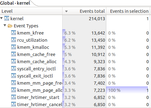
The view is separated in two sides. The left side of the view presents the Statistics in a table. The table shows 3 columns: Level Events total and Events in selected time range. The data is organized per trace. After parsing a trace the view will display the number of events per event type in the second column and in the third, the currently selected time range's event type distribution is shown. The cells where the number of events are printed also contain a colored bar with a number that indicates the percentage of the event count in relation to the total number of events.
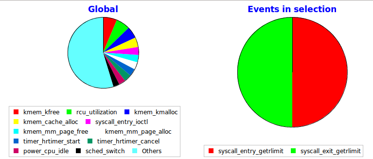
The right side illustrates the proportion of types of events into two pie charts. The legend of each pie chart gives the representation of each color in the chart.
By default, the statistics use a state system, therefore will load very quickly once the state system is written to the disk as a supplementary file.
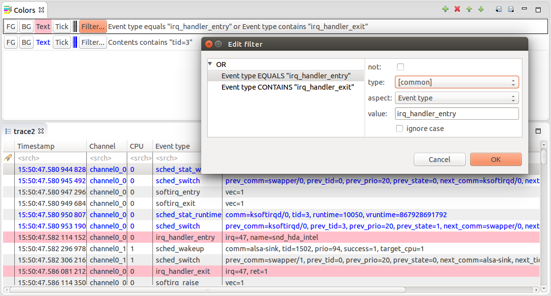
The Colors view allows the user to define a prioritized list of color settings.
A color setting associates a foreground and background color (used in any events table), and a tick color (used in the Time Chart view), with an event filter.
In an events table, any event row that matches the event filter of a color setting will be displayed with the specified foreground and background colors. If the event matches multiple filters, the color setting with the highest priority will be used.
The same principle applies to the event tick colors in the Time Chart view. If a tick represents many events, the tick color of the highest priority matching event will be used.
Color settings can be inserted, deleted, reordered, imported and exported using the buttons in the Colors view toolbar. Changes to the color settings are applied immediately, and are persisted to disk.
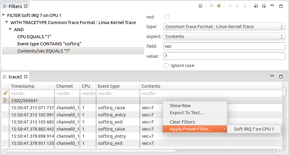
The Filters view allows the user to define preset filters that can be applied to any events table.
The filters can be more complex than what can be achieved with the filter header row in the events table. The filter is defined in a tree node structure, where the node types can be any of TRACETYPE, AND, OR, CONTAINS, EQUALS, MATCHES or COMPARE. Some nodes types have restrictions on their possible children in the tree.
The TRACETYPE node filters against the trace type of the trace as defined in a plug-in extension or in a custom parser. When used, any child node will have its type combo box fixed and its aspect combo box restricted to the possible aspects of that trace type. Depending of the Trace Types enabled in the Trace Types preference page, the list of available trace types for the filtering can vary.
The AND node applies the logical and condition on all of its children. All children conditions must be true for the filter to match. A not operator can be applied to invert the condition.
The OR node applies the logical or condition on all of its children. At least one children condition must be true for the filter to match. A not operator can be applied to invert the condition.
The CONTAINS node matches when the specified event aspect value contains the specified value string. A not operator can be applied to invert the condition. The condition can be case sensitive or insensitive. The type combo box restricts the possible aspects to those of the specified trace type.
The EQUALS node matches when the specified event aspect value equals exactly the specified value string. A not operator can be applied to invert the condition. The condition can be case sensitive or insensitive. The type combo box restricts the possible aspects to those of the specified trace type.
The MATCHES node matches when the specified event aspect value matches against the specified regular expression. A not operator can be applied to invert the condition. The type combo box restricts the possible aspects to those of the specified trace type.
The COMPARE node matches when the specified event aspect value compared with the specified value gives the specified result. The result can be set to smaller than, equal or greater than. The type of comparison can be numerical, alphanumerical or based on time stamp. A not operator can be applied to invert the condition. The type combo box restricts the possible aspects to those of the specified trace type.
For numerical comparisons, strings prefixed by "0x", "0X" or "#" are treated as hexadecimal numbers and strings prefixed by "0" are treated as octal numbers.
For time stamp comparisons, strings are treated as seconds with or without fraction of seconds. This corresponds to the TTT format in the Time Format preferences. The value for a selected event can be found in the Properties view under the Timestamp property. The common 'Timestamp' aspect can always be used for time stamp comparisons regardless of its time format.
Filters can be added, deleted, imported and exported using the buttons in the Filters view toolbar. The nodes in the view can be Cut (Ctrl-X), Copied (Ctrl-C) and Pasted (Ctrl-V) by using the buttons in the toolbar or by using the key bindings. This makes it easier to quickly build new filters from existing ones. Changes to the preset filters are only applied and persisted to disk when the Save filters button is pressed.
To apply a saved preset filter in an events table, right-click on the table and select Apply preset filter... > filter name.
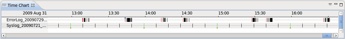
The Time Chart view allows the user to visualize every open trace in a common time chart. Each trace is display in its own row and ticks are display for every punctual event. As the user zooms using the mouse wheel or by right-clicking and dragging in the time scale, more detailed event data is computed from the traces. The time axis is aligned with other views that support automatic time axis alignment (see Automatic Time Axis Alignment).
Time synchronization is enabled between the time chart view and other trace viewers such as the events table.
Color settings defined in the Colors view can be used to change the tick color of events displayed in the Time Chart view.
When a search is applied in the events table, the ticks corresponding to matching events in the Time Chart view are decorated with a marker below the tick.
When a bookmark is applied in the events table, the ticks corresponding to the bookmarked event in the Time Chart view is decorated with a bookmark above the tick.
When a filter is applied in the events table, the non-matching ticks are removed from the Time Chart view.
The Time Chart only supports traces that are opened in an editor. The use of an editor is specified in the plug-in extension for that trace type, or is enabled by default for custom traces.
The
Align Views toggle button
in the view menu allows to disable and enable the automatic time axis alignment of time-based views. Disabling the alignment in the this view will disable this feature across all the views because it's a workspace preference.
The State System Explorer view allows the user to inspect the state interval values of every attribute of a state system at a particular time.
The view shows a tree of currently selected traces and their registered state system IDs. For each state system the tree structure of attributes is displayed. The attribute name, quark, value, start and end time, and full attribute path are shown for each attribute.
To modify the time of attributes shown in the view, select a different current time in other views that support time synchronization (e.g. event table, histogram view). When a time range is selected, this view uses the begin time.
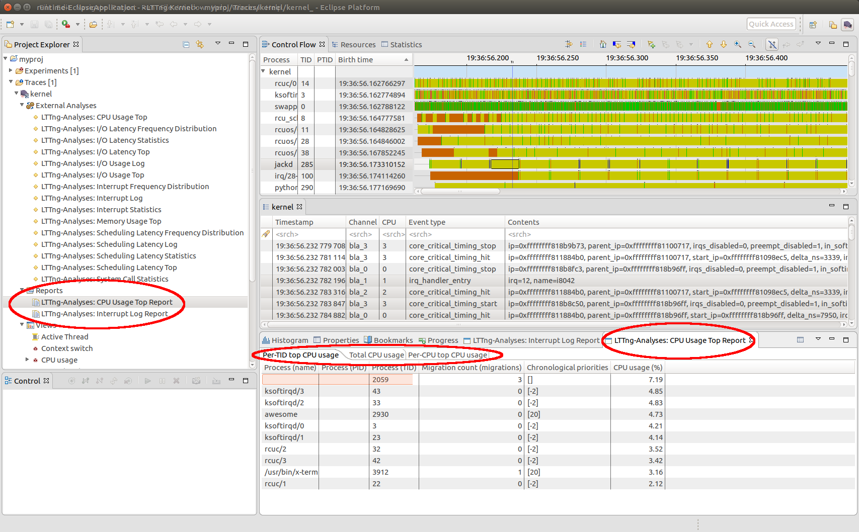
Trace Compass supports the execution of external analyses conforming to the LAMI 1.0.x specification. This includes recent versions of the LTTng-Analyses project.
An external analysis is a program executed by Trace Compass. When the program is done analyzing, Trace Compass generates a report containing its results. A report contains one or more tables which can also be viewed as bar and scatter charts.
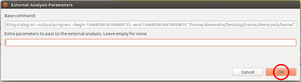
Note: The program to execute is found by searching the directories listed in the standard $PATH environment variable when no path separator (/ on Unix and OS X, \ on Windows) is found in its command.
Trace Compass ships with a default list of descriptors of external analyses (not the analyses themselves), including the descriptors of the LTTng analyses. If the LTTng analyses project is installed, its analyses are available when opening or importing an LTTng kernel trace.
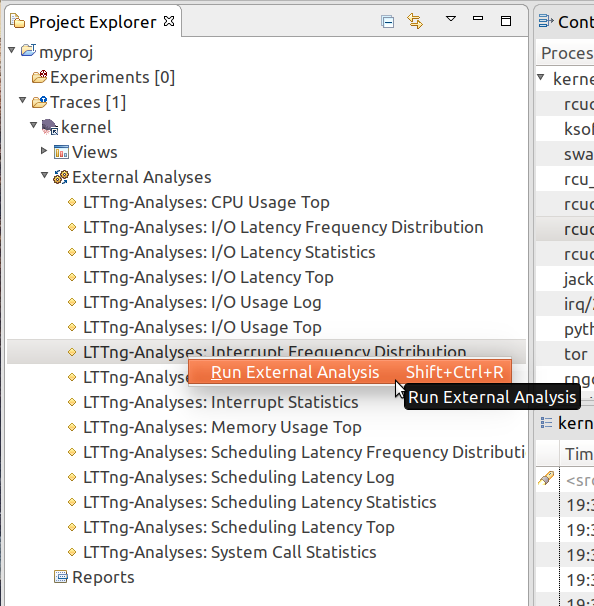
To run an external analysis:
The external analyses which are either missing or not compatible with the trace are stroke and cannot be executed.
You can use views like the Histogram View and the Control Flow View (if it's available for this trace) to make a time range selection.
External analyses are executed on the current time range selection if there is one, or on the whole trace otherwise.
Note that many external analyses can be started concurrently.
When the external analysis is done analyzing, its results are saved as a report in Trace Compass. The tables contained in this report are also automatically opened into a new report view when the analysis is finished.
A report is created after a successful execution of an external analysis.
To open a report:
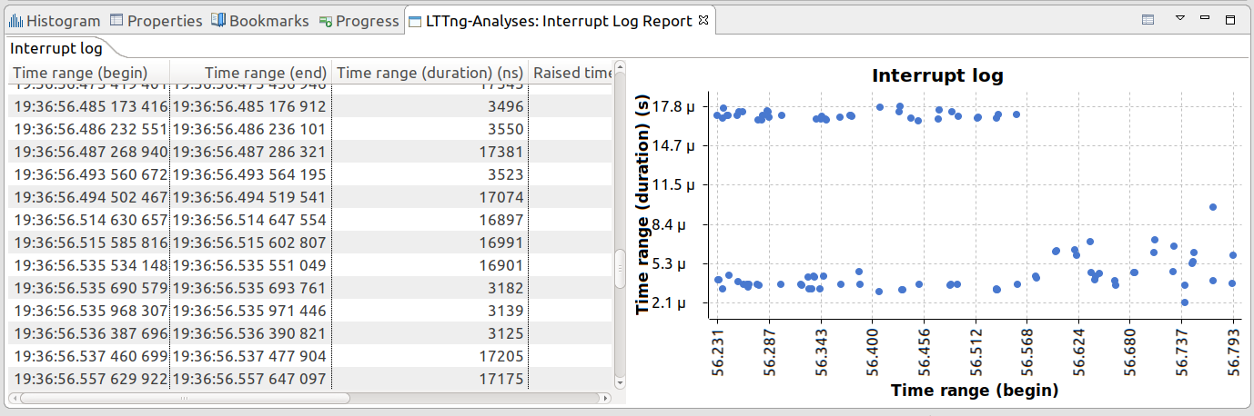
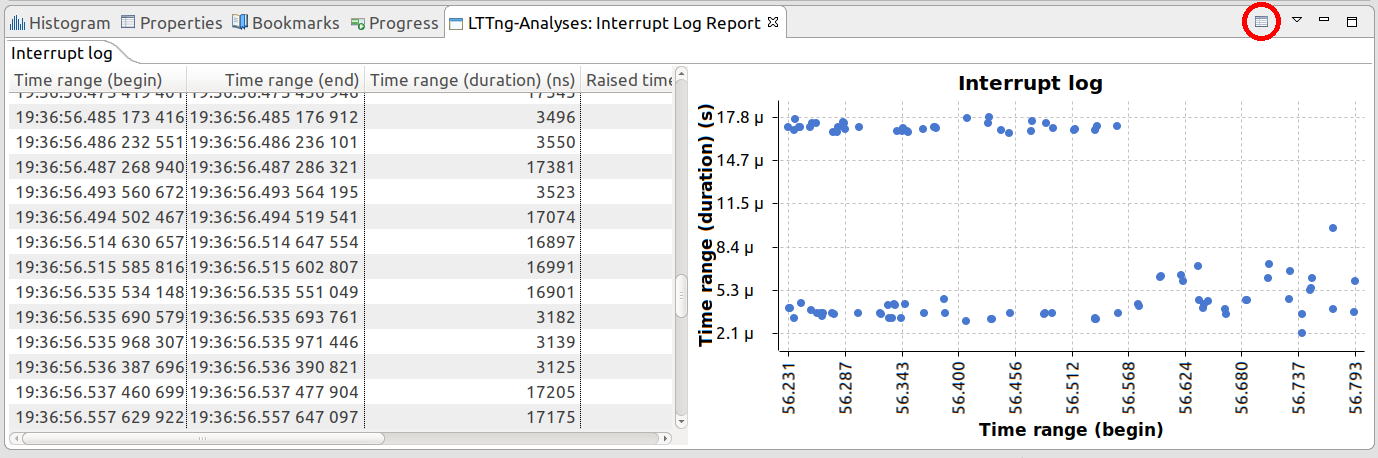
Each result table generated by the external analysis is shown in its own tab in the opened report view.
To create a bar or a scatter chart from the data of a given result table:
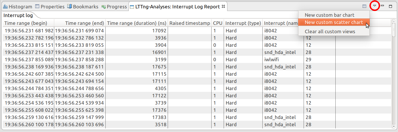
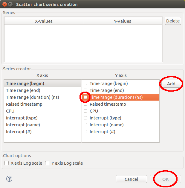
Repeat this step to create more series.
The chart is created and shown at the right of its source result table.
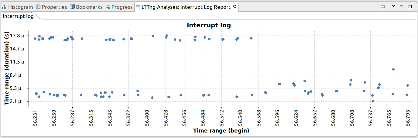
To show or hide a result table once a chart has been created:
If the result table was visible, it is now hidden:
You can add a user-defined external analysis to the current list of external analyses. Note that the command to invoke must conform to the machine interface of LTTng analyses 0.4.
Note: If you want to create your own external analysis, consider following the LAMI 1.0 specification, which is supported by later versions of Trace Compass.
To add a user-defined external analysis:
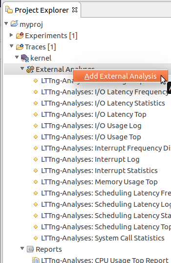
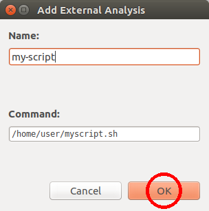
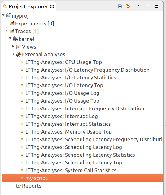
The name is the title of the external analysis as shown under External Analyses in the Project Explorer View.
The command is the complete command line to execute. You can put arguments containing spaces or other special characters in double quotes.
Note: If the command is not a file system path, then it must be found in the directories listed in the $PATH environment variable.
A user-defined external analysis with a green icon is created under External Analyses in the Project Explorer View.
Note: The new external analysis entry is saved in the workspace.
To remove a user-defined external analysis:
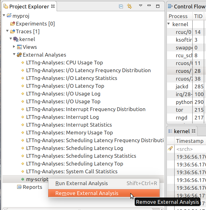
Note: Only user-defined (green icon) external analyses can be removed.
Custom parser wizards allow the user to define their own parsers for text or XML traces. The user defines how the input should be parsed into internal trace events and identifies the event fields that should be created and displayed. Traces created using a custom parser can be correlated with other built-in traces or traces added by plug-in extension.
The New Custom Text Parser wizard can be used to create a custom parser for text logs. It can be launched several ways:
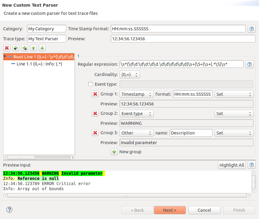
Fill out the first wizard page with the following information:
Note: information about date and time patterns can be found here: TmfTimestampFormat
Click the Add next line, Add child line or Remove line buttons to create a new line of input or delete it. For each line of input, enter the following information:
Note: information about regular expression patterns can be found here: https://docs.oracle.com/javase/8/docs/api/java/util/regex/Pattern.html
Important note: The custom parsers identify a log entry when the first line's regular expression matches (Root Line n). Each subsequent text line in the log is attempted to be matched against the regular expression of the parser's input lines in the order that they are defined (Line n.*). Only the first matching input line will be used to process the captured data to be stored in the log entry. When a text line matches a Root Line's regular expression, a new log entry is started.
Click the Add group or Remove group buttons to define the data extracted from the capturing groups in the line's regular expression. For each group, enter the following information:
The Preview input text box can be used to enter any log data that will be processed against the defined custom parser. When the wizard is invoked from a selected log file resource, this input will be automatically filled with the file contents.
The Preview: text field of each capturing group and of the Time Stamp will be filled from the parsed data of the first matching log entry.
In the Preview input text box, the matching entries are highlighted with different colors:
Yellow : indicates uncaptured text in a matching line. Green : indicates a captured group in the matching line's regular expression for which a custom parser group is defined. This data will be stored by the custom parser. Magenta : indicates a captured group in the matching line's regular expression for which there is no custom parser group defined. This data will be lost. White : indicates a non-matching line.The first line of a matching entry is highlighted with darker colors.
By default only the first matching entry will be highlighted. To highlight all matching entries in the preview input data, click the Highlight All button. This might take a few seconds to process, depending on the input size.
Click the Next > button to go to the second page of the wizard.
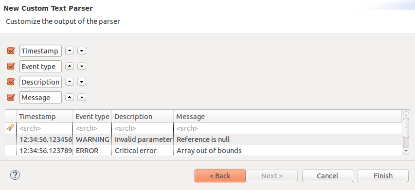
On this page, the list of default and custom data is shown, along with a preview of the custom parser log table output.
The custom data output can be modified by the following options:
The table at the bottom of the page shows a preview of the custom parser log table output according to the selected options, using the matching entries of the previous page's Preview input log data.
Click the Finish button to close the wizard and save the custom parser.
The New Custom XML Parser wizard can be used to create a custom parser for XML logs. It can be launched several ways:
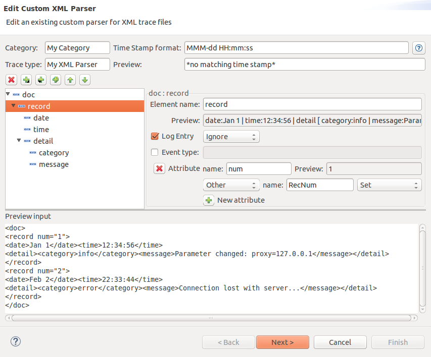
Fill out the first wizard page with the following information:
Note: information about date and time patterns can be found here: TmfTimestampFormat
Click the Add document element button to create a new document element and enter a name for the root-level document element of the XML file.
Click the Add child button to create a new element of input to the document element or any other element. For each element, enter the following information:
Note: An element's extracted data 'value' is a parsed string representation of all its attributes, children elements and their own values. To extract more specific information from an element, ignore its data value and extract the data from one or many of its attributes and children elements.
Click the Add attribute button to create a new attribute input from the document element or any other element. For each attribute, enter the following information:
Note: A log entry can inherited input data from its parent elements if the data is extracted at a higher level.
Click the Feeling lucky button to automatically and recursively create child elements and attributes for the current element, according to the XML element data found in the Preview input text box, if any.
Click the Remove element or Remove attribute buttons to remove the extraction of this input data. Take note that all children elements and attributes are also removed.
The Preview input text box can be used to enter any XML log data that will be processed against the defined custom parser. When the wizard is invoked from a selected log file resource, this input will be automatically filled with the file contents.
The Preview: text field of each capturing element and attribute and of the Time Stamp will be filled from the parsed data of the first matching log entry. Also, when creating a new child element or attribute, its element or attribute name will be suggested if possible from the preview input data.
Click the Next > button to go to the second page of the wizard.
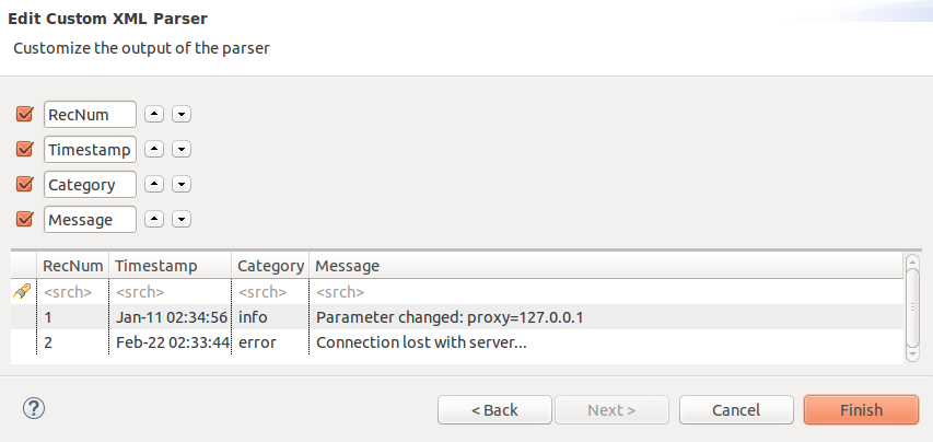
On this page, the list of default and custom data is shown, along with a preview of the custom parser log table output.
The custom data output can be modified by the following options:
The table at the bottom of the page shows a preview of the custom parser log table output according to the selected options, using the matching entries of the previous page's Preview input log data.
Click the Finish button to close the wizard and save the custom parser.
The Manage Custom Parsers dialog is used to manage the list of custom parsers used by the tool. To open the dialog:
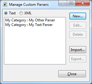
The ordered list of currently defined custom parsers for the selected type is displayed on the left side of the dialog.
To change the type of custom parser to manage, select the Text or XML radio button.
The following actions can be performed from this dialog:
Click the New... button to launch the New Custom Parser wizard.
Select a custom parser from the list and click the Edit... button to launch the Edit Custom Parser wizard.
Select a custom parser from the list and click the Delete button to remove the custom parser.
Click the Import... button and select a file from the opened file dialog to import all its custom parsers. If any parser conflicts with an existing built-in or custom trace type, the user will be prompted to skip or rename the imported parser.
Select a custom parser from the list, click the Export... button and enter or select a file in the opened file dialog to export the custom parser. Note that if an existing file containing custom parsers is selected, the custom parser will be appended to the file.
Once a custom parser has been created, any imported trace file can be opened and parsed using it.
To do so:
The trace will be opened in an editor showing the events table, and an entry will be added for it in the Time Chart view.
Some views, such as time graph and XY chart views, can be opened multiple times in order to show content from different traces and/or window ranges simultaneously. This can be done by using the New <view name> view sub-menu in the view's View Menu at the far right of the tool bar.
By default, a view shows content from the active trace, which is the last trace whose events editor tab has been selected.
When a view is pinned, it no longer follows the active trace and is locked to the trace to which it is pinned. The view's tab will show the pinned trace's name within brackets, e.g. View Name < trace name >.
A view can be pinned to the current active trace by clicking the
Pin View button
 on the tool bar, or pinned to any specific opened trace by using the
Pin View button's drop-down menu. This drop-down menu can also be used to switch the pinned trace of a pinned view. Once a view is pinned, it can be unpinned by clicking the
Unpin View button
on the tool bar, or pinned to any specific opened trace by using the
Pin View button's drop-down menu. This drop-down menu can also be used to switch the pinned trace of a pinned view. Once a view is pinned, it can be unpinned by clicking the
Unpin View button
 on the tool bar.
or select
Pin to <first trace> from its button drop-down menu
or select
Pin to <trace> from its button drop-down menu
All time-based views that show the same trace are synchronized in time to show the same window range and time selection. This also applies to the selected event(s) in the Events Editor.
By default, changing the window range or time selection for one trace does not affect the window range or time selection of other opened traces.
To allow a specific trace to be synchronized with (and react to) the window range or time selection from other traces, check the Follow time updates from other traces toggle option in that trace's Event Editor context menu. This does not affect whether this trace's time updates will be propagated to other traces.
Time synchronization will only occur if the updated window range or time selection from the other trace overlaps with the full time range of the following trace. It will occur even if the following trace is not the active trace.
Note that two opened instances of the same trace are never time synchronized with each other, regardless of the toggle option.
Trace Compass supports automatic alignment of the time axis for time-based views. The user now can resize the time window of one view and all other open views will align to the new window size and position. The automatic alignment is optional and can be disabled and enabled using the Align Views button of the view menu. Disabling or enabling it in one view it will disable and enable it for all view since it's a workspace wide setting.
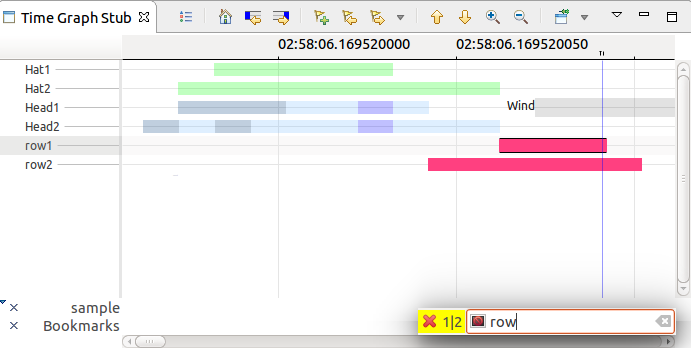
Search for an entry in a Time Graph view, e.g. Control Flow View or Resources View, using the Find dialog. To use the dialog:
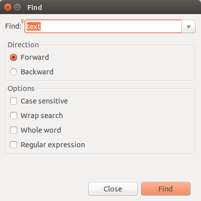
Various options are available in the Options group:
The Direction group allows to select the search direction: Forward or Backward .
Filtering time events in a Time Graph view, e.g. Control Flow View or Resources View, using the Time Event Filter dialog box. To do so:
Note that Regular expression is supported.
It is possible to save multiple filters. They will be all activated at the same time in the view. To save a filter:
Note that user can still use the dialog box to filter the remaining visible time events in the view.
Note that the view has a limit of 4 saved filters.
Note that all links are dimmed when a filter is applied and completely removed when there is active saved filters.
To remove a saved filter, click on the remove button next to the filter.
The time event filtering uses its own domain-specific language (DSL) . Various logical operators are suppported:
Filter expressions have the following pattern field operator argument in general. Several relational operators are available:
Filter expressions can have the following pattern field operator . The available relational operators for this pattern is:
The DSL allows the possibility to realize complex filters, combining several Filter expressions and using parenthesis. Example: TID != 5755 && (System_call contains select)
Note that field parameter with whitespace should be specified using quotes mark. Example: "SOFT IRQ" present
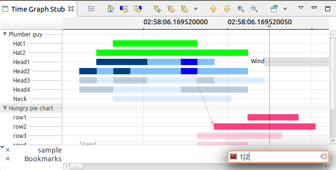
Time Graph Views support filtering of empty rows using a dynamic filter. Empty rows are rows with no time events nor row markers in the current visible time range. To hide empty rows, check the
![]() Hide Empty Rows toolbar button or view menu entry. Unchecking it will show empty rows again. When changing the current visible time range, the list of visible rows will be dynamically updated.
Hide Empty Rows toolbar button or view menu entry. Unchecking it will show empty rows again. When changing the current visible time range, the list of visible rows will be dynamically updated.
Time graph views can allow the user to display periodic markers over time graphs by selecting a marker set. The marker sets are user-configurable by editing the markers.xml file.
From the view menu, select Marker Set > Edit.... The markers.xml file will be opened in an editor. After editing the file, save the modifications, and then select Marker Set > marker set name to activate the marker set. Select Marker set > None to deactivate the marker set.
The format of the markers.xml file is defined as follows:
<marker-sets> (marker-set*)
  <market-set> (marker*)
    <marker> ((submarker | segments))*
      <submarker> ((submarker | segments))*
      </submarker>
      <segments> (segment+, ((submarker | segments))*)
        <segment/> ((submarker | segments))*
      </segments>
    </marker>
  </marker-set>
</marker-sets>
The <marker> element defines a fixed-period marker at the root of the marker set. Optionally, a <marker> can have child <submarker> elements, which split each marker into a number of equal sub-markers, and/or child <segments> elements, which split each marker into segments of defined weights defined by the list of child <segment> elements. Each of these elements can recursively have their own <submarker> and <segments> child elements.
The element attributes are defined as follows:
<marker-set name="name" id="id">
<marker name="name" label="label" id="id" referenceid="referenceid" color="color" period="period" unit="unit" range="range" offset="offset" index="index">
<submarker name="name" label="label" id="id" color="color" range="range" index="index">
<segments name="name">
<segment label="label" id="id" color="color" length="length">
An example marker set configuration can be found below:
<?xml version="1.0" encoding="UTF-8"?>
<marker-sets xmlns:xsi="http://www.w3.org/2001/XMLSchema-instance" xsi:noNamespaceSchemaLocation="markers.xsd">
	<marker-set name="Example" id="example.id">
		<marker name="Frame" color="#ff0000" period="10" unit="ms" range="0..4095">
			<submarker name="Subframe" color="#00ff00" label="#%d Normal" range="0..9" index="0,2..9">
				<submarker name="Slot" color="#008800" range="0..1"/>
			</submarker>
			<submarker name="Subframe" color="#ff8800" label="#%d Special" range="0..9" index="1">
				<segments name="Slot">
					<segment label="A" color="#884400" length="1"/>
					<segment label="B" color="#884400" length="3"/>
					<segment label="C" color="#884400" length="2"/>
				</segments>
			</submarker>
		</marker>
	</marker-set>
</marker-sets>
|
|

|
|
| Installation | LTTng Tracer Control |